Reductive Groups Part II: Over More General Fields

In Reductive Groups Part I: Over Algebraically Closed Fields we learned about how reductive groups over algebraically closed fields are classified by their root datum, and how the based root datum helps us understand their automorphisms. In this post, we consider reductive groups over more general, not necessarily algebraically closed fields. We will discuss how they can be classified, and also define the Langlands dual of a reductive group, which will allow us to state the local Langlands correspondence (see The Local Langlands Correspondence for General Linear Groups) for certain groups other than just the general linear group.

Let F be a field. We will say an algebraic group G over F is a reductive group if G_{\overline{F}}, the base change of G to the algebraic closure \overline{F}, is a reductive group. Similarly, we say that G is a torus if the base change G_{\overline{F}} is a torus. This means that after base change to the algebraic closure it becomes isomorphic to the product of copies of the multiplicative group \mathbb{G}_{m}. However, if over F it is already isomorphic to the product of copies of \mathbb{G}_{m}, without the need for a base change, then we say that it is a split torus. If a reductive group G contains a maximal split torus, we say that G is split. We note that a “maximal split torus” is different from a “split maximal torus”!

The classification of split reductive groups is the same as that of reductive groups over algebraically closed fields – they are classified by their root datum. As such they will provide us with the first step towards classifying reductive groups over more general fields.

If G is a reductive group over F, a form of G is some other reductive group G' over F such that after base change to the algebraic closure \overline{F}, G_{\overline{F}} and G_{\overline{F}} are isomorphic. It happens that any reductive group is a form of a split reductive group. This follows from the fact that any abstract root datum is the root datum associated to some reductive group and some split maximal torus contained in it.

The forms of a split group are classified using Galois cohomology. Suppose we have an isomorphism f:G_{\overline{F}}\simeq G_{\overline{F}}. The Galois group \mathrm{Gal}(\overline{F}/F) (henceforth shortened to just \mathrm{Gal}_{F}) acts on the isomorphism f by conjugation, giving rise to another isomorphism ^{\sigma}f:G_{\overline{F}}\simeq G_{\overline{F}}'. Composing this with the inverse of f we get an automorphism f^{-1}\circ^{\sigma}f of G_{\overline{F}}. This automorphism is an example of a 1cocycle in Galois cohomology.

More generally, in Galois cohomology, for some group M with a Galois action (for instance in our case M=\mathrm{Aut}(G)_{\overline{F}})), a 1-cocycle is a homomorphism \varphi:\mathrm{Gal}_{F}\to M such that \varphi(\sigma\tau)=\varphi(\sigma)\cdot^{\sigma}\varphi(\tau). Two 1-cocycles \varphi, \psi are cohomologous if there is an element m\in M such that \psi(\sigma)=m^{-1}\varphi(\sigma)^{\sigma}m. The set of 1-cocycles, modulo those which are cohomologous, is denoted H^{1}(\mathrm{Gal}_{F},M).

By the above construction there is a map between the set of isomorphism classes of forms of G and the Galois cohomology group H^{1}(\mathrm{Gal}_{F},\mathrm{Aut}(G_{\overline{F}})). This map actually happens to be a bijection!

Let BR be a based root datum corresponding to G together with a pinning. We have mentioned in Reductive Groups Part I: Over Algebraically Closed Fields the group of automorphisms of BR, the pinned automorphisms of G, and the outer automorphisms of G are all isomorphic to each other. We have the following exact sequence

\displaystyle 0\to\mathrm{Inn}(G_{\overline{F}})\to\mathrm{Aut}(G_{\overline{F}})\to\mathrm{Out}(G_{\overline{F}})\to 0

and when we are provided the additional data of a pinning this gives us a splitting of the exact sequence (i.e. a way to decompose the middle term into a semidirect product of the other two terms).

When the pinning is defined over F, we obtain a homomorphism

\displaystyle H^{1}(\mathrm{Gal}_{F},\mathrm{Aut}(G_{\overline{F}}))\to H^{1}( \mathrm{Gal}_{F}, \mathrm{Out}(G_{\overline{F}}))

where H^{1}(\mathrm{Gal}_{F}, \mathrm{Out}(G_{\overline{F}})) is in bijection with the set of conjugacy classes of group homomorphisms \mu:\mathrm{Gal}_{F}\to \mathrm{Out}(G_{\overline{F}}). But we have said earlier that H^{1}(\mathrm{Gal}_{F},\mathrm{Aut}(G_{\overline{F}})) is in bijection with the set of isomorphism classes of forms of G. Therefore, any form of G gives us such a homomorphism \mu:\mathrm{Gal}_{F}\to \mathrm{Out}(G_{\overline{F}}).

We say that a reductive group is quasi-split if it contains a Borel subgroup. Split reductive groups are automatically quasi-split.

An inner form of a reductive group G is another reductive group G' related by an isomorphism f:G_{\overline{F}}\simeq G_{\overline{F}}' such that the composition f^{-1}\circ^{\sigma}f is an inner automorphism of G_{\overline{F}}.

Once we have a split group G, and given the data of a pinning, we can now use any morphism \mu:\mathrm{Gal}_{F}\to\mathrm{Out}(G) together with the given pinning to obtain an element of H^{1}(\mathrm{Gal}_{F},\mathrm{Aut}(G_{\overline{F}})), which in turn will give us a quasi-split form of G. Now it happens that any reductive group G has a unique quasi-split inner form!

Therefore, in summary, the classification of reductive groups over general fields proceeds in the following three steps:

  1. Classify the split reductive groups using the root datum.
  2. Classify the quasi-split forms using the homomorphisms \mathrm{Gal}_{F}\to\mathrm{Out}(G).
  3. Classify the inner forms of the quasi-split forms.

Let us now discuss the Langlands dual (also known as the L-group) of a reductive group. Since every abstract root datum corresponds to some reductive group G (say, over a field F), we can interchange the roots and coroots and get another reductive group \widehat{G}, which we refer to as the dual group of G.

The Langlands dual of G is the group (an honest to goodness group, not an algebraic group) given by the semidirect product \widehat{G}(\mathbb{C})\rtimes \mathrm{Gal}_{F}. In order to construct this semidirect product we need an action of \mathrm{Gal}_{F} on \widehat{G}(\mathbb{C}), and in this case this action is via its action on the based root datum of \widehat{G} together with a Borel subgroup B\subseteq G, which is the same as a pinned automorphism of \widehat{G}. We denote the Langlands dual of G by ^{L}G.

Let us recall that in The Local Langlands Correspondence for General Linear Groups we stated the local Langlands correspondence, in the case of \mathrm{GL}_{n}(F) where F is a local field, as a correspondence between the irreducible admissible representations of \mathrm{GL}_{n}(F) (over \mathbb{C}) and the F-semisimple Weil-Deligne representations of the Weil group W_{F} of F.

With the definition of the Langlands dual in hand, we can now state the local Langlands correspondence more generally, not just for \mathrm{GL}_{n}(F), and in this case it will not even be a one-to-one correspondence between irreducible admissible representations and Weil-Deligne representations anymore!

First, we will need the notion of a Langlands parameter, also called an L-parameter, which takes the place of the F-semisimple Weil-Deligne representation. It is defined to be a continuous homomorphism W_{F}\times \mathrm{SL}_{2}(\mathbb{C})\to ^{L}G such that, as a homomorphism from W_{F} to ^{L}G, it is semisimple, the composition W_{F}\to^{L}G\to\mathrm{Gal}_{F} is just the usual inclusion of W_{F} into \mathrm{Gal}_{F}, and as a function of \mathrm{SL}_{2}(\mathbb{C}) to \widehat{G}(\mathbb{C}) it comes from a morphism of algebraic groups from \mathrm{SL}_{2} to \widehat{G}.

And now for the statement: The local Langlands correspondence states that, for a reductive group G over a local field F, the irreducible admissible representations of G(F) are partitioned into a finite disjoint union of sets, called L-packets, labeled by (equivalence classes of, where the equivalence is given by conjugation by elements of \widehat{G}(\mathbb{C})) L-parameters. In other words, letting \mathrm{Irr}_{G} be the set of isomorphism classes of irreducible admissible representations of G, and letting \Phi be the set of equivalence classes of L-parameters, we have

\mathrm{Irr}_{G}=\coprod_{\phi\in\Phi}\Pi_{\phi}

where \Pi_{\phi} is the L-packet, a set of irreducible admissible representations of G(F). In the case that F is p-adic and G=\mathrm{GL}_{n}, each of these L-packets have only one element and this reduces to the one-to-one correspondence which we saw in The Local Langlands Correspondence for General Linear Groups.

The L-group and L-parameters are also expected to play a part in the global Langlands correspondence (in the case of function fields over a finite field, the construction of L-parameters was developed by Vincent Lafforgue using excursion operators). There is also much fascinating theory connecting the representations of the L-group to the geometry of a certain geometric object constructed from the original reductive group called the affine Grassmannian. We will discuss more of these topics in the future.

References:

Reductive group on Wikipedia

Root datum on Wikipedia

Inner form on Wikipedia

Langlands dual group on Wikipedia

Topics in automorphic forms (notes by Chao Li from a course by Jack Thorne)

Representation theory and number theory (notes by Chao Li from a course by Benedict Gross)

Algebraic groups by J. S. Milne

Formal Schemes

In Galois Deformation Rings we discussed the dual numbers as well as the concept of deformations. The dual numbers are numbers with an additional “tangent direction” or a “derivative” – we can further take into account higher order derivatives to consider deformations, which leads us to the concept of deformations.

In this post, we will consider spaces related to deformations, called formal schemes. Let us begin with a motivating example. Consider a field k. From algebraic geometry, we know that the underlying topological space of the scheme \mathrm{Spec}(k) is just a single point. What about the dual numbers, which is the ring k[x]/(x^{2}). What is the underlying topological space of the scheme \mathrm{Spec}(k[x]/(x^{2}))? It turns out it is also just the point!

So as far as the underlying topological spaces go, there is no difference between \mathrm{Spec}(k) and \mathrm{Spec}(k[x]/(x^{2})) – they are both just points. This is because they both have one prime ideal. For k this is the ideal (0), which is also its only ideal that is not itself. For k[x]/(x^{2}), its one prime ideal is the ideal (x); note that the ideal (0) in k[x]/(x^{2}) is not prime, which is related to this ring not being an integral domain. However a scheme is more than just its underlying topological space, one also has the data of its structure sheaf, i.e. its ring of regular functions, and in this regard \mathrm{Spec}(k) and \mathrm{Spec}(k[x]/(x^{2})) are different.

We sometimes consider \mathrm{Spec}(k[x]/(x^{2})) as a “thickening” of \mathrm{Spec}(k) – they are both just the point, but the functions on \mathrm{Spec}(k[x]/(x^{2})) have derivatives, as if there were tangent directions on the point that is the underlying space of \mathrm{Spec}(k[x]/(x^{2})) on which one can move “infinitesimally”, unlike on the point that is the underlying space of \mathrm{Spec}(k).

Just like in our discussion in Galois Deformation Rings, we may want to consider not only the “first-order derivatives” which appear in the dual numbers but also “higher-order derivatives”; we may even want to consider all of them together. This amounts to taking the inverse limit \varprojlim_{n}k[x]/(x^{n}), which is the formal power series ring k[[x]]. However, if we take \mathrm{Spec}(k[[x]]), we will see that it actually has two points, a “generic point” (corresponding to the ideal (0), which is prime because k[[x]] is an integral domain) and a “special point” (corresponding to the ideal (x), which is also prime and furthermore the lone maximal ideal), unlike \mathrm{Spec}(k) or \mathrm{Spec}(k[x]/(x^{2})) (or more generally \mathrm{Spec}(k[x])/(x^{n})), for any n, justified by similar reasons to the preceding argument).

This is where formal schemes come in – a formal scheme can express the “thickening” of some other scheme, with all the “higher-order derivatives”, where the underlying topological space is the same as that of the original scheme but the structure sheaf might be different, to reflect this “thickening”.

A topological ring is a ring A equipped with a topology such that the usual ring operations are continuous with respect to this topology. In this post we will mostly consider the I-adic topology, for some ideal I called the ideal of definition. This topology is generated by a basis consisting of sets of the form a+I^{n}, for a in A.

An example of a topological ring with the I-adic topology is the formal power series ring k[[x]] which we have discussed, together with the ideal of definition (x). Another example is the p-adic integers \mathbb{Z}_{p}, together with the ideal of definition (p). We note that all these examples are complete with respect to the I-adic topology.

More generally for higher dimension one can take, say, an affine variety cut out by some polynomial equation, say y^{2}=x^{3}, and consider the ring k[x,y]/(y^{2}-x^{3}). Note that \mathrm{Spec}(k[x,y]/(y^{2}-x^{3})) is an affine variety. Now we can form a topological ring complete with respect to the I-adic topology, by taking the completion with respect to the ideal I=(y^{2}-x^{3}), i.e. the inverse limit of the diagram

\displaystyle k[x,y]/(y^{2}-x^{3})\leftarrow  k[x,y]/(y^{2}-x^{3})^{2} \leftarrow  k[x,y]/(y^{2}-x^{3})^{3} \leftarrow\ldots

The formation of this ring is an important step in describing the “thickening” of the affine variety \mathrm{Spec}(k[x,y]/(y^{2}-x^{3})), but as said above, it cannot just be done by taking the “spectrum”. Therefore we introduce the idea of a formal spectrum.

Let A be a Noetherian topological ring and let I be an ideal of definition. In addition, let A be complete with respect to the I-adic topology. We define the formal spectrum of A, denoted \mathrm{Spf}(A), to be the pair (X,\mathcal{O}_{X}), where X is the underlying topological space of \mathrm{Spec}(A/I), and the structure sheaf \mathcal{O}_{X} is defined by setting \mathcal{O}_{X}(D_{f}) to be the I-adic completion of A[1/f], for D_{f} the distinguished open set corresponding to f. Applied to the examples earlier, this gives us what we want – a sort of “thickening” of some affine scheme, with an underlying topological space the same as that of the original scheme but with a structure sheaf of functions with “higher-order derivatives”.

More generally, to include the “non-affine” case a formal scheme is a topologically ringed space, i.e. a pair (X,\mathcal{O}_{X}) where X is a topological space and \mathcal{O}_{X} is a sheaf of topological rings, such that for any point x of X there is an open neighborhood of x which is isomorphic as a topologically ringed space to \mathrm{Spf}(A) for some Noetherian topological ring A.

Aside from being useful in deformation theory, formal schemes are also related to rigid analytic spaces (see also Rigid Analytic Spaces). For certain types of formal schemes (“locally formally of finite type over \mathrm{Spf}(\mathbb{Z}_{p})“) one can assign (functorially) a rigid analytic space. For example, this functor will assign to the formal scheme \mathrm{Spf}(\mathbb{Z}_{p}[[x]]) the open unit disc (the interior of the closed unit disc in Rigid Analytic Spaces). This functor is called the generic fiber functor, which is an odd name, because \mathrm{Spf}(\mathbb{Z}_{p}[[x]]) has no “generic points”! However, there is a way to make this name make more sense using the language of adic spaces, which also subsumes the theory of both formal schemes and rigid analytic spaces, and also provides a natural home for the perfectoid spaces we hinted at in Perfectoid Fields. The theory of adic spaces will hopefully be discussed in some future post on this blog.

References:

Formal Scheme on Wikipedia

Berkeley Lectures on p-adic Geometry by Peter Scholze and Jared Weinstein

Modular Curves at Infinite Level by Jared Weinstein

Adic Spaces by Jared Weinstein

Algebraic Geometry by Robin Hartshorne

p-adic Hodge Theory: An Overview

In The Theory of Motives we discussed the notion of a Weil cohomology, and mentioned four “classical” examples, the singular (also known as Betti) cohomology, the de Rham cohomology, the \ell-adic cohomology, and the crystalline cohomology.

Cohomology theories may be thought of as a way to study geometric objects using linear algebra, by associating vector spaces (or more generally, modules or abelian groups) to such a geometric object. But the four Weil cohomology theories above actually give more than just a vector space:

  • The singular cohomology has an action of complex conjugation.
  • The de Rham cohomology has a Hodge filtration.
  • The \ell-adic cohomology has an action of the Galois group.
  • The crystalline cohomology has an action of Frobenius (and a Hodge filtration as well).

There are relations between these different cohomologies. For example, for a smooth projective variety X over the complex numbers \mathbb{C}, the singular cohomology of the corresponding complex analytic manifold X(\mathbb{C}), with complex coefficients (this can be obtained from singular cohomology with integral coefficients by tensoring with \mathbb{C}) and the de Rham cohomology are isomorphic:

\displaystyle H_{\mathrm{sing}}^{k}(X(\mathbb{C}),\mathbb{Z})\otimes_{\mathbb{Z}}\mathbb{C}=H_{\mathrm{dR}}^{k}(X)

The roots of this idea go back to de Rham’s work on complex manifolds, where chains in singular homology (which is dual to singular cohomology, see also Homology and Cohomology) can be paired with the differential forms of de Rham cohomology (see also Differential Forms), simply by integrating the differential forms along these chains. By the machinery developed by Alexander Grothendieck, this can be ported over into the world of algebraic geometry.

Again borrowing from the world of complex manifolds, the machinery of Hodge theory gives us the following Hodge decomposition (see also Shimura Varieties):

\displaystyle H_{\mathrm{sing}}^{k}(X(\mathbb{C}),\mathbb{Z})\otimes_{\mathbb{Z}}\mathbb{C}=\bigoplus_{i+j=k} H^{i}(X,\Omega_{X/\mathbb{C}}^{j})

Now again for the case of smooth projective varieties over the complex numbers , \ell-adic cohomology also has such an isomorphism with singular cohomology – but this time if it has \ell-adic coefficients (i.e. in \mathbb{Q}_{\ell}).

\displaystyle H_{\mathrm{sing}}^{k}(X(\mathbb{C}),\mathbb{Z})\otimes_{\mathbb{Z}}\mathbb{Q}_{\ell}\simeq H_{\mathrm{et}}^{k}(X,\mathbb{Q}_{\ell})

Such isomorphisms are also known as comparison isomorphisms (or comparison theorems).
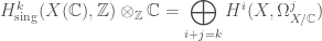
More generally, if we have a field B into which we can embed both \mathbb{Q}_{\ell} and \mathbb{C} (for instance \mathbb{C}), we obtain the following comparison theorem:

\displaystyle  H_{\mathrm{et}}^{k}(X,\mathbb{Q}_{\ell}) \otimes_{\mathbb{Q_{\ell}}} B\simeq  H_{\mathrm{dR}}^{k}(X) \otimes_{\mathbb{C}} B

Here is a very interesting thing that these comparison theorems can give us. Let X be a modular curve. Then the Hodge decomposition for the first cohomology gives us

\displaystyle H_{\mathrm{sing}}^{1}(X(\mathbb{C}),\mathbb{Z})\otimes_{\mathbb{Z}}\mathbb{C}=H^{1}(X,\Omega_{X/\mathbb{C}}^{0})\oplus H^{0}(X,\Omega_{X/\mathbb{C}}^{1})

But the H^{0}(X,\Omega_{X/\mathbb{C}}^{1}) is the cusp forms of weight 2 as per the discussion in Modular Forms (see also Galois Representations Coming From Weight 2 Eigenforms). By the results of Hodge theory, the other summand H^{1}(X,\Omega_{X/\mathbb{C}}^{0}) is just the complex conjugate of H^{0}(X,\Omega_{X/\mathbb{C}}^{1}). But we now also have a comparison with etale cohomology, which has a Galois representation! For this the modular form must lie in the cohomology with \mathbb{Q} coefficients, which happens if it is a Hecke eigenform whose Hecke eigenvalues are in \mathbb{Q}. So one of the great things that these comparison theorems gives us is this way of relating modular forms and Galois representations.

The comparison isomorphisms above work for smooth projective varieties over the complex numbers, but let us now go to the p-adic world, and let us consider smooth projective varieties over the p-adic numbers.

It was observed by John Tate (and later explored by Gerd Faltings) that the p-adic cohomology (i.e. the etale cohomology of a smooth projective variety over \mathbb{Q}_{p}, or more generally some other p-adic field, with p-adic coefficients, distinguishing it from \ell-adic cohomology where another prime \ell different from p must be brought in) can have a decomposition akin to the Hodge decomposition, after tensoring it with the p-adic complex numbers (this is the completion of the algebraic closure of the p-adic numbers):

\displaystyle H^{k}(X_{\overline{\mathbb{Q}}_{p}},\mathbb{Q}_{p})\otimes_{\mathbb{Q}_{p}}\mathbb{C}_{p}=\bigoplus_{i+j=k} H^{i}(X,\Omega_{X/\mathbb{Q}}^{j})\otimes_{\mathbb{Q}}\mathbb{C}_{p}(-j)

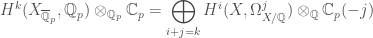
The p-adic complex numbers here play the role of the complex numbers in the singular cohomology case above or the \ell-adic numbers in the \ell-adic case.

The ideas conjectured by Tate, and later completed by Faltings, was but the prototype of what is now known as p-adic Hodge theory. In its modern form, p-adic Hodge theory concerns comparison isomorphisms between different Weil cohomology theories on smooth projective varieties over the p-adic numbers. However, the role played by the complex numbers, \ell-adic numbers (for the complex case), and p-adic complex numbers (for the p-adic case) must now be played by much more complicated objects called period rings, which were developed by Jean-Marc Fontaine. We will discuss the construction of the period rings at the end of this post, but first let us see how they work.

Let X be a smooth projective variety over \mathbb{Q}_{p} (or more generally some other p-adic field). Let H_{\mathrm{dR}}^{i}(X) and H_{\mathrm{et}}^{i}(X_{\overline{\mathbb{Q}}_{p}},\mathbb{Q}_{p}) be its de Rham cohomology and the p-adic etale cohomology of its base change to the algebraic closure \overline{\mathbb{Q}}_{p} respectively. The comparison isomorphism at the center of p-adic Hodge theory is the following:
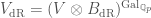
\displaystyle H_{\mathrm{dR}}^{i}(X)\otimes_{\mathbb{Q}_{p}} B_{\mathrm{dR}}=H_{\mathrm{et}}^{i}(X_{\overline{\mathbb{Q}}_{p}},\mathbb{Q}_{p})\otimes_{\mathbb{Q}_{p}} B_{\mathrm{dR}}

The object denoted B_{\mathrm{dR}} here is the aforementioned period ring. It is equipped with both a Galois action and a filtration akin to the Hodge filtration. More than just that isomorphism above, we also have a way of obtaining the de Rham cohomology if we are given the p-adic etale cohomology, simply by taking the part that is invariant under the Galois action:

\displaystyle  \displaystyle H_{\mathrm{dR}}^{i}(X)=(H_{\mathrm{et}}^{i}(X_{\overline{\mathbb{Q}}_{p}},\mathbb{Q}_{p})\otimes_{\mathbb{Q}_{p}} B_{\mathrm{dR}})^{\mathrm{Gal}_{\mathbb{Q}_{p}}}

To go the other way, i.e. to recover the p-adic etale cohomology from the de Rham cohomology, we will need a different kind of period ring. This period ring is B_{\mathrm{cris}}, which aside from having a Galois action and a filtration also has an action of Frobenius. Aside from providing us the same isomorphism between de Rham and p-adic etale cohomology upon tensoring, it also provides us with a solution to our earlier problem (as long as X has a smooth proper integral model) as follows:

\displaystyle H_{\mathrm{et}}^{i}(X_{\overline{\mathbb{Q}}_{p}},\mathbb{Q}_{p})= \mathrm{Fil}^{0}(H_{\mathrm{dR}}^{i}(X)\otimes_{\mathbb{Q}_{p}} B_{\mathrm{cris}})^{\varphi=1}

This idea can be further abstracted – since etale cohomology provides Galois representations, we can just take some p-adic Galois representation instead, without caring whether it comes from etale cohomology or not, and tensor it with a period ring, then take Galois invariants. For instance let V be some p-adic Galois representation. Then we can take the tensor product

V_{\mathrm{dR}}=(V\otimes B_{\mathrm{dR}})^{\mathrm{Gal}_{\mathbb{Q}_{p}}}

If the dimension of V_{\mathrm{dR}} is equal to the dimension of V, then we say that the Galois representation V is de Rham. Similarly we can tensor with B_{\mathrm{cris}}:

V_{\mathrm{cris}}=(V\otimes B_{\mathrm{cris}})^{\mathrm{Gal}_{\mathbb{Q}_{p}}}

If its V_{\mathrm{cris}} is equal to the dimension of V , we say that V is crystalline.

The idea of these “de Rham” and “crystalline” Galois representations is that if they come from the corresponding cohomologies then they will have these properties. But does the converse hold? If they are “de Rham” and “crystalline” does that mean that they come from the corresponding cohomologies (i.e. they “come from geometry”)? This is roughly the content of the Fontaine-Mazur conjecture.

Now let us say a few things about the construction of these period rings. These constructions make use of the concepts we discussed in Perfectoid Fields. We start with the ring A_{\mathrm{inf}}(\mathcal{O}_{\mathbb{C}_{p}}), which, as we recall from Perfectoid Fields, is the ring of Witt vectors of the tilt of \mathcal{O}_{\mathbb{C}_{p}}. By inverting p and taking the completion with respect to the canonical map \theta:  A_{\mathrm{inf}}(\mathcal{O}_{\mathbb{C}_{p}}) \to\mathcal{O}_{\mathbb{C}_{p}}
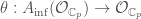
, we obtain a ring which we suggestively denote by B_{\mathrm{dR}}^{+}.

There is a special element t of B_{\mathrm{dR}}^{+} which we think of as the logarithm of the element (1, \zeta^{1/p},\zeta^{1/p},\ldots). Upon inverting this element t, we obtain the field B_{\mathrm{dR}}.

The field B_{\mathrm{dR}} is equipped with a Galois action, carried over from the fields involved in its construction, and a filtration, given by \mathrm{Fil}^{i}B_{\mathrm{dR}}=t^{i}B_{\mathrm{dR}}.

To construct B_{\mathrm{cris}}, we once again start with A_{\mathrm{inf}}(\mathcal{O}_{\mathbb{C}_{p}}) and invert p. However, to have a Frobenius, instead of completing with respect to the kernel of the map \theta, we take a generator of this kernel (which we shall denote by \omega). Then we denote by B_{\mathrm{cris}}^{+} the ring formed by all the power series of the form \sum_{n=0}^{\infty} a_{n}\omega^{n}/n! where the a_{n}‘s are elements of A_{\mathrm{inf}}(\mathcal{O}_{\mathbb{C}_{p}})[1/p] which converge as n\to\infty, under the topology of A_{\mathrm{inf}}(\mathcal{O}_{\mathbb{C}_{p}})[1/p] (which is not the p-adic topology!). Once again there will be an element t like before; we invert t to obtain B_{\mathrm{cris}}.

There is yet another period ring called B_{\mathrm{st}}, where the subscript stands for semistable; in addition to a Galois action, filtration, and Frobenius, it has a monodromy operator. Since this is less extensively discussed in introductory literature, we follow this lead and leave this topic, and the many other wonderful topics related to p-adic Hodge theory, to future posts on this blog.

References:

p-adic Hodge theory on Wikipedia

de Rham cohomology on Wikipedia

Hodge theory on Wikipedia

An invitation to p-adic Hodge theory, or: How I learned to stop worrying and love Fontaine by Alex Youcis

Seminar on the Fargues-Fontaine curve (Lecture 1 – Overview) by Jacob Lurie

An introduction to the theory of p-adic representations by Laurent Berger

Reciprocity laws and Galois representations: recent breakthroughs Jared Weinstein

Reductive Groups Part I: Over Algebraically Closed Fields

In many posts on this blog we have talked about elliptic curves, which are examples of algebraic groups (which is itself a specific instance of a group scheme) – a variety whose points form a group. As varieties, elliptic curves (and abelian varieties in general) are projective. There are also algebraic groups which are affine, and in this post we will discuss a special class of affine algebraic groups, called reductive groups, which as we shall see are related to many familiar objects, and are well-studied. In particular, in the case when they are defined over algebraically closed fields we will discuss their classification in terms of root datum. We will also discuss how this root datum helps us understand the automorphisms of such a reductive group.

An example of a reductive group is \mathrm{GL}_{n}; let’s assume that this is a variety defined over some field F. If R is some F-algebra, then the R-valued points of \mathrm{GL}_{n} (in the “functor of points” point of view) is the group \mathrm{GL}_{n}(R) of n\times n matrices with nonzero determinant. Geometrically, we may think of the nonzero determinant condition as the polynomial equation that cuts out the variety \mathrm{GL}_{n}.

Linear algebraic groups are smooth closed algebraic subgroups of \mathrm{GL}_{n}, and they have their own “representation theory”, a “representation” in this context being a morphism from some linear algebraic group G to the algebraic group \mathrm{GL}(V), for some vector space V over some field E. The algebraic group \mathrm{GL}(V) is the algebraic group whose R-valued points give the group of linear transformations of the E-vector space R\otimes V.

A linear algebraic group is a reductive group if it is geometrically connected and every representation is semisimple (a direct product of irreducible representations).

We also denote the reductive group \mathrm{GL}_{1} by \mathbb{G}_{m}. A torus is a reductive group which is isomorphic to a product of copies of \mathbb{G}_m. A torus contained in a reductive group G is called maximal if it is not contained in some strictly larger torus contained in G.

Let T be a maximal torus of the reductive group G. The Weyl group (G,T) is the quotient N(T)/Z(T) where N(T) is the normalizer of T in G (the subgroup consisting of all elements g in G such that for any element t in T gtg^{-1} is an element of T) and Z(T) is the centralizer of T in G (the subgroup consisting of all elements in G that commute with all the elements of T).

Now let us discuss the classification of reductive groups, for which we will need the concept of roots and root datum.

For a maximal torus T in a reductive group G, the characters (homomorphisms from T to \mathbb{G}_{m}) and the cocharacters (homomorphisms from T to \mathbb{G}_{m}) will play an important role in this classification. Let us denote the characters of T by X^{*}(T), and the cocharacters of T by X_{*}(T).

Just like Lie groups, reductive groups have a Lie algebra (the tangent space to the identity), on which it acts (therefore giving a representation of the reductive group, called the adjoint representation). We may restrict to a maximal torus T contained in the reductive group G, so that the Lie algebra \mathfrak{g} of G gives a representation of T. This gives us a decomposition of \mathfrak{g} as follows:

\displaystyle \mathfrak{g}=\mathfrak{g}_{0}\oplus \bigoplus_{\alpha}\mathfrak{g}_{\alpha}

Here \mathfrak{g}_{\alpha} is the subspace of \mathfrak{g} on which T acts as a character \alpha:T\to\mathbb{G}_{m}. The nonzero characters \alpha for which \mathfrak{g}_{\alpha} is nonzero are called roots. We denote the set of roots by \Phi.

For a character \alpha, let T_{\alpha} be the connected component of the kernel of \alpha. Let G_{\alpha} be the centralizer of T_{\alpha} in G. Then the Weyl group W(G_{\alpha},T) will only have two elements, the identity and one other element, which we shall denote by s_{\alpha}. There will be a unique cocharacter \alpha^{\vee} satisfying the equation

s_{\alpha}(x)=x-\langle \alpha^{\vee},x\rangle\alpha

for all characters x:T\to\mathbb{G}_{m}. This cocharacter is called a coroot. We denote the set of coroots by \Phi^{\vee}.

The datum (\Phi, X^{*}(T), \Phi^{\vee}, X_{*}(T)) is called the root datum associated to G. This root datum is actually independent of the chosen maximal torus, which follows from all maximal tori being contained in a unique conjugacy class in G.

There is also a concept of an “abstract” root datum, a priori having seemingly nothing to do with reductive groups, just some datum (M, \Psi, M^{\vee}, \Psi^{\vee}) where M and M^{\vee} are finitely generated abelian groups, \Psi is a subset of M\setminus \lbrace 0\rbrace, and \Psi^{\vee} is a subset of M^{\vee}\setminus \lbrace 0\rbrace, and they satisfy the following axioms:

  • There is a perfect pairing \langle,\rangle:M\times M^{\vee}\to\mathbb{Z}.
  • There is a bijection between \Psi and \Psi^{\vee}.
  • For any \alpha\in \Psi, and \alpha^{\vee} its image in \Psi under the aforementioned bijection, we have \langle \alpha,\alpha^{\vee}\rangle=2.
  • For any \alpha\in \Psi, the automorphism of M given by x\mapsto \alpha-\langle x,\alpha^{\vee}\rangle\alpha preserves \alpha.
  • The subgroup of \mathrm{Aut}(M) generated by x\mapsto \alpha-\langle x,\alpha^{\vee}\rangle\alpha is finite.

Again, a priori, such a datum of finitely generated abelian groups and their subsets, satisfying these axioms, seems to have nothing to do with reductive groups. However, we have the following amazing theorem:

Any abstract root datum is the root datum associated to some reductive group.

For reductive groups over an algebraically closed field, the root datum classifies reductive groups:

Two reductive groups over an algebraically closed field have the same root datum if and only if they are isomorphic.

Let us now discuss how root datum helps us understand the automorphisms of a reductive group. For this we need to expand the information contained in the root datum.

A root basis is a subset of the roots such that any root can be expressed as a unique linear combination of the roots, where the integer coefficients are either all positive or all negative. A based root datum is given by (\Phi, X^{*}(T), S, \Phi^{\vee}, X_{*}(T), S^{\vee}), i.e. the usual root datum together with the additional datum of a root basis S.

The root datum already determines the reductive group G. What does the additional data of a root basis mean? The root basis corresponds to a Borel subgroup of G that contains our chosen maximal torus T. A Borel subgroup of G is a maximal connected solvable Zariski closed algebraic subgroup of G.

A pinning is the datum (G,T,B,\lbrace x_{\alpha}\rbrace_{\alpha\in S}) where T is a maximal torus, B is a Borel subgroup containing T, and \lbrace x_{\alpha}\rbrace_{\alpha\in S} is a basis element of \mathfrak{g}_{\alpha}. Given a pinning, a pinned automorphism of G is an automorphism of G that preserves the pinning.

An inner automorphism of a group G is one that comes from conjugation by some element; in a way they are the automorphisms that are easier to understand. The inner automorphisms form a normal subgroup \mathrm{Inn}(G) of the group of automorphisms \mathrm{Aut}(G), and the quotient \mathrm{Aut}(G)/\mathrm{Inn}(G) is called \mathrm{Out}(G). We have similar notions for algebraic groups.

Now a pinned automorphism is an automorphism, therefore has a map to \mathrm{Out}(G). A pinned automorphism also has a map to the automorphisms of the corresponding based root datum. Both of these maps are actually isomorphisms! Therefore we have a description of \mathrm{Aut}(G) as follows:

The automorphisms of G as an algebraic group are given by the semidirect product of the inner automorphisms and the automorphisms of the based root datum.

In this post we have only focused on the case of reductive groups over algebraically closed fields. Over more general fields the theory of reductive groups, for instance the classification, is more complicated. This will hopefully be tackled in future posts on this blog.

References:

Algebraic group on Wikipedia

Linear algebraic group on Wikipedia

Reductive group on Wikipedia

Root datum on Wikipedia

Topics in automorphic forms (notes by Chao Li from a course by Jack Thorne)

Representation theory and number theory (notes by Chao Li from a course by Benedict Gross)

Lectures on the geometry and modular representation theory of algebraic groups by Geordie Williamson and Joshua Ciappara

Algebraic groups by J. S. Milne

Rigid Analytic Spaces

This blog post is inspired by and follows closely an amazing talk given by Ashwin Iyengar at the “What is a…seminar?” online seminar. I hope I can do the talk, and this wonderful topic, some justice in this blog post.

One of the most fascinating and powerful things about algebraic geometry is how closely tied it is to complex analysis, despite what the word “algebraic” might lead one to think. To state one of the more simple and common examples, we have that smooth projective curves over the complex numbers \mathbb{C} are the same thing as compact Riemann surfaces. In higher dimensions we also have Chow’s theorem, which tells us that an analytic subspace of complex projective space which is topologically closed is an algebraic subvariety.

This is all encapsulated in what is known as “GAGA“, named after the foundational work “Géometrie Algébrique et Géométrie Analytique” by Jean-Pierre Serre. We refer to the references at the end of this post for the more precise statement, but for now let us think of GAGA as giving us a fully faithful functor from proper algebraic varieties over \mathbb{C} to complex analytic spaces, which gives us an equivalence of categories between their coherent sheaves.

One may now ask if we can do something similar with the p-adic numbers \mathbb{Q}_{p} (or more generally an extension K of \mathbb{Q}_{p} that is complete with respect to a valuation that extends the one on \mathbb{Q}_{p}) instead of \mathbb{C}. This leads us to the theory of rigid analytic spaces, which was originally developed by John Tate to study a p-adic version of the idea (also called “uniformization”) that elliptic curves over \mathbb{C} can be described as lattices on \mathbb{C}.

Let us start defining these rigid analytic spaces. If we simply naively try to mimic the definition of complex analytic manifolds by having these rigid analytic spaces be locally isomorphic to \mathbb{Q}_{p}^{m}, with analytic transition maps, we will run into trouble because of the peculiar geometric properties of the p-adic numbers – in particular, as a topological space, the p-adic numbers are totally disconnected!

To fix this, we cannot just use the naive way because the notion of “local” would just be too “small”, in a way. We will take a cue from algebraic geometry so that we can use the notion of a Grothendieck topology to fix what would be issues if we were to just use the topology that comes from the p-adic numbers.

The Tate algebra \mathbb{Q}_{p}\langle T_{1},\ldots,T_{n}\rangle is the algebra formed by power series in n variables that converge on the n-dimensional unit polydisc D^{n}, which is the set of all n-tuples (c_{1},\ldots,c_{n}) of elements of \mathbb{Q}_{p} that have p-adic absolute value less than or equal to 1 for all i from 1 to n.

There is another way to define the Tate algebra, using the property of power series with coefficients in p-adic numbers that it converges on the unit polydisc D^{n} if and only if its coefficients go to zero (this is not true for real numbers!). More precisely if we have a power series

\displaystyle f(T_{1},\ldots,T_{n})=\sum_{a} c_{a}T_{1}^{a_{1}}\ldots T_{n}^{a_{n}}

where c_{a}\in \mathbb{Q}_{p} and a=a_{1}+\ldots+a_{n} runs over all n-tuples of natural numbers, then f converges on the unit polydisc D^{n} if and only if \lim_{a\to 0}c_{a}=0.

The Tate algebra has many important properties, for example it is a Banach space (see also Metric, Norm, and Inner Product) with the norm of an element given by taking the biggest p-adic absolute value among its coefficients. Another property that will be very important in this post is that it satisfies a Nullstellensatz – orbits of the absolute Galois group \mathrm{Gal}(\overline{\mathbb{Q}}_{p}/\mathbb{Q}_{p}) in D^{n} correspond to maximal ideals of the Tate algebra. Explicitly, this correspondence is given by the evaluation map x\in D^{n}\mapsto \lbrace f\vert f(x)=0\rbrace.

A quotient of the Tate algebra by some ideal is referred to as an affinoid algebra. The maximal ideals of the underlying set of an affinoid algebra A will be denoted \mathrm{Max}(A), and this should be reminiscent of how we obtain the closed points of a scheme.

Once we have the underlying set \mathrm{Max}(A) , we need two other things to be able to define “affinoid” rigid analytic spaces, which we shall later “glue” to form more general rigid analytic spaces – a topology, and a structure sheaf (again this should be reminiscent of how schemes are defined).

Again taking a cue from how schemes are defined, we define “rational domains”, which are analogous to the distinguished Zariski open sets of (the underlying topological space of) a scheme. Given elements f_{1},\ldots,f_{r},g of the affinoid algebra A, the rational domain \displaystyle A\left(\frac{f}{g}\right) is the set of all x\in\mathrm{Max}(A) such that f_{i}(x)\leq g(x) for all 1\leq i\leq r.

The rational domains generate a topology, however this is still just the p-adic topology, and so it still does not solve the problems that we originally ran into when we tried to define rigid analytic spaces by mimicking the definition of a complex analytic manifold. The trick will be to make use of something that is more general than just a topology – a Grothendieck topology (see also More Category Theory: The Grothendieck Topos).

Let us now define the particular Grothendieck topology that we will use. Unlike other examples of a Grothendieck toplogy, the covers will involve only subsets of the space being covered (it is also referred to as a mild Grothendieck topology). Let X=\mathrm{Max}(A). A subset U of X is called an admissible open if it can be covered by rational domains \lbrace U_{i}\rbrace_{i\in I} such that for any map Y\to X where Y=\mathrm{Max}(B) for some affinoid algebra B, the covering of Y given by the inverse images of the U_{i}‘s admit a finite subcover.

If U is an admissible open covered by admissible opens \lbrace U_{i}\rbrace_{i\in I}, then this covering is called admissible if for any map Y\to X whose image is contained in U, the covering of Y given by the inverse images of the U_{i}‘s admit a finite subcover. These admissible coverings satisfy the axioms for a Grothendieck topology, which we denote G_{X}.

If A is an affinoid algebra, and f_{1},\ldots,f_{k},g are functions, we let \displaystyle A\left\langle \frac{f}{g}\right\rangle denote the ring A\langle T_{1},\ldots T_{k}\rangle/(gT_{i}-f_{i}). By associating to a rational domain \displaystyle A\left(\frac{f}{g}\right) this ring \displaystyle A\left\langle\frac{f}{g}\right\rangle, we can define a structure sheaf \cal{O}_{X} on this Grothendieck topology.

The data consisting of the set X=\mathrm{Max}(A), the Grothendieck topology G_{X}, and the structure sheaf \mathcal{O}_{X} is what makes up an affinoid rigid analytic space. Finally, just as with schemes, we define a more general rigid analytic space as the data consisting of some set X, a Grothendieck topology G_{X} and a sheaf \mathcal{O}_{X} such that locally, with respect to the Grothendieck topology G_{X}, it is isomorphic to an affinoid rigid analytic space.

Under this definition, we have in fact a version of GAGA that holds for rigid analytic spaces – a fully faithful functor from proper schemes of finite type over \mathbb{Q}_{p} to rigid analytic spaces over \mathbb{Q}_{p} that gives an equivalence of categories between their coherent sheaves.

Finally let us now look at an example. Consider the affinoid rigid analytic space obtained from the affinoid algebra \mathbb{Q}_{p}\langle T\rangle. By the Nullstellensatz the underlying set is the unit disc D. The “boundary” of this is the rational subdomain (and therefore an admissible open) \displaystyle D\left(\frac{1}{T}\right), and its complement, the “interior” is covered by rational subdomains \displaystyle D\left(\frac{T^{n}}{p}\right). With this covering the interior may also be shown to be an admissible open.

While it appears that, since we found two complementary admissible opens, we can disconnect the unit disc, we cannot actually do this in the Grothendieck topology, because the set consisting of the boundary and the interior is not an admissible open! And so in this way we see that the Grothendieck topology is the difference maker that allows us to overcome the obstacles posed by the peculiar geometry of the p-adic numbers.

Since Tate’s innovation, the idea of a p-adic or nonarchimedean geometry has blossomed with many kinds of “spaces” other than the rigid analytic spaces of Tate, for example adic spaces, a special class of which generalize perfectoid fields (see also Perfectoid Fields) to spaces, or Berkovich spaces, which are honest to goodness topological spaces instead of relying on a Grothendieck topology like rigid analytic spaces do. Such spaces will be discussed on this blog in the future.

References:

Rigid analytic space on Wikipedia

Algebraic geometry and analytic geometry on Wikipedia

Several approaches to non-archimedean geometry by Brian Conrad

Reciprocity laws and Galois representations: recent breakthroughs by Jared Weinstein

p-adic families of modular forms [after Coleman, Hida, and Mazur] by Matthew Emerton