In The Global Langlands Correspondence for Function Fields over a Finite Field, we introduced the global Langlands correspondence for function fields over a finite field, and Vincent Lafforgue’s work on the automorphic to Galois direction of the correspondence. In this post we will discuss the work of Laurent Fargues and Peter Scholze which uses similar ideas but applies it to the local Langlands correspondence (and this time it works not only for “equal characteristic” cases like Laurent series fields  but also for “mixed characteristic” cases like finite extensions of
  ). Note that instead of having complex coefficients like in The Local Langlands Correspondence for General Linear Groups, here we will use
  -adic coefficients.
I. The Fargues-Fontaine Curve
Let us briefly discuss the idea of “geometrization” and what is meant by Fargues and Scholze making use of V. Lafforgue’s work. Recall that V. Lafforgue’s work concerns the global Langlands correspondence for function fields over a finite field  , which on one side concerns the space of cuspidal automorphic forms, which are certain functions on
  , which in turn parametrizes
  -bundles on some curve
  over , and on the other side concerns representations (or more precisely L-parameters) of the etale fundamental group of (which can also be phrased in terms of the Galois group of its function field).
Perhaps the first question that comes to mind is, what is the analogue of the curve in the case of the local Langlands correspondence when the field is not a function field (or more correctly a power series field, since it has to be local) over , but some finite extension of ? Let  be this finite extension of . Since the absolute Galois group of is also the etale fundamental group of
  , perhaps we should take to be our analogue of .
However, in the traditional formulation of the local Langlands correspondence, it is the Weil group that appears instead of the absolute Galois group itself. Considering the theory of the Weil group in Weil-Deligne Representations, this means that we will actually want  , where
  is the maximal unramified extension of and
  is the Frobenius, instead of
  .
.
Now, we want to “relativize” this. For instance, in The Global Langlands Correspondence for Function Fields over a Finite Field, we considered , which parametrizes -bundles on the curve over . But we may also want to consider say  , where
  is some -algebra; this would parametrize -bundles on
  instead. In fact, we need this “relativization” to properly define
  as a stack (see also Algebraic Spaces and Stacks).
The problem with transporting this to the case of a finite extension of is that we do not have an “base” like was for the function field case (unless perhaps if we have something like an appropriate version of the titular object in The Field with One Element, which is at the moment unavailable). The solution to this is provided by the theory of adic spaces and perfectoid spaces (see also Adic Spaces and Perfectoid Spaces).
For motivation, let us consider first the case where our field is . Let  be a perfectoid space over
  with pseudouniformizer
  . Consider the product
  . We may look at this as the punctured open unit disc over
  . It sits inside
 ![\mathrm{Spa}(R^{+})\times_{\mathrm{Spa}(\mathbb{F}_{q})}\mathrm{Spa}(\mathbb{F}_{q}[[t]])](https://s0.wp.com/latex.php?latex=%5Cmathrm%7BSpa%7D%28R%5E%7B%2B%7D%29%5Ctimes_%7B%5Cmathrm%7BSpa%7D%28%5Cmathbb%7BF%7D_%7Bq%7D%29%7D%5Cmathrm%7BSpa%7D%28%5Cmathbb%7BF%7D_%7Bq%7D%5B%5Bt%5D%5D%29&bg=ffffff&fg=444444&s=0&c=20201002) as the locus where the pseudo-uniformizer
as the locus where the pseudo-uniformizer  of and the uniformizer
  of
of ![\mathbb{F}_{q}[[t]]](https://s0.wp.com/latex.php?latex=%5Cmathbb%7BF%7D_%7Bq%7D%5B%5Bt%5D%5D&bg=ffffff&fg=444444&s=0&c=20201002) is invertible (or “nonzero”).
is invertible (or “nonzero”).
In the case where our field is , a finite extension of , as mentioned earlier we have no “base” like was for . So we cannot form the fiber products analogous to or . However, notice that
![\displaystyle \mathrm{Spa}(R^{+})\times_{\mathrm{Spa}(\mathbb{F}_{q})}\mathrm{Spa}(\mathbb{F}_{q}[[t]])\cong \mathrm{Spa}(R^{+}[[t]])](https://s0.wp.com/latex.php?latex=%5Cdisplaystyle+%5Cmathrm%7BSpa%7D%28R%5E%7B%2B%7D%29%5Ctimes_%7B%5Cmathrm%7BSpa%7D%28%5Cmathbb%7BF%7D_%7Bq%7D%29%7D%5Cmathrm%7BSpa%7D%28%5Cmathbb%7BF%7D_%7Bq%7D%5B%5Bt%5D%5D%29%5Ccong+%5Cmathrm%7BSpa%7D%28R%5E%7B%2B%7D%5B%5Bt%5D%5D%29&bg=ffffff&fg=444444&s=0&c=20201002) .
.
This has an analogue in the mixed-characteristic, given by the theory of Witt vectors (compare, for instance ![\mathbb{F}_{p}[[t]]](https://s0.wp.com/latex.php?latex=%5Cmathbb%7BF%7D_%7Bp%7D%5B%5Bt%5D%5D&bg=ffffff&fg=444444&s=0&c=20201002) and its “mixed-characteristic analogue”
and its “mixed-characteristic analogue”  )! If
)! If  is the residue field of
  , we define the ramified Witt vectors
  to be
to be  . This is the analogue of . Now all we have to do to find the analogue of that we are looking for is to define it as the locus in where both the uniformizer of
  and the uniformizer of are invertible!
We denote this locus by  . But recall again our discussion earlier, that due to the local Langlands correspondence being phrased in terms of the Weil group, we have to quotient out by the powers of Frobenius. Therefore we define the Fargues-Fontaine curve
  to be
to be  .
.
Aside from our purpose of geometrizing the local Langlands correspondence, the Fargues-Fontaine curve is in itself a very interesting mathematical object. For instance, when is a complete algebraically closed nonarchimedean field over , the classical points of (i.e. maximal ideals of the rings  such that is locally
  ) correspond to untilts of (modulo the action of Frobenius)!
There is also a similar notion for more general . To explain this we need the concept of diamonds, which will also be very important for the rest of the post. A diamond is a pro-etale sheaf on the category of perfectoid spaces over  , which is the quotient of some perfectoid space over
  by a pro-etale equivalence relation
  (we also say that the diamond is a coequalizer). An example of a diamond is given by
  . Note that is not perfectoid, but is the quotient of a perfectoid field we denoted
  in Adic Spaces and Perfectoid Spaces by the action of
  . Now we can take the tilt
  and quotient out by
  (the underline notation will be explained later – for now we think of this as making the group into a perfectoid space) – this is the diamond . More generally, if is an adic space over
  satisfying certain conditions (“analytic”), we can define the diamond
  to be such that
  , for a perfectoid space over , is the set of isomorphism classes of pairs
  ,
,  being the untilt of . If
  , we also use
  to denote . Note that if is already perfectoid, is just the same thing as the tilt
  .
.
Now recall that was defined to be the locus in  where the uniformizer of and the uniformizer of were invertible. We actually have that
  , and, for the Fargues-Fontaine curve , we have that
  .
.
Our generalization of the statement that the points of parametrize untilts of is now as follows. There exists a three-way bijection between sections of the map  , maps
  , and untilts over of . Given such an untilt , this defines a closed Cartier divisor on , which in turn gives rise to a closed Cartier divisor on . By the bijection mentioned earlier, these closed Cartier divisors on will be parametrized by maps
  .
.
The closed Cartier divisors that arise in this way will be referred to as closed Cartier divisors of degree  . We have seen that they are parametrized by the following moduli space we denote by
  (this will also become important later on):
Now that we have discussed the Fargues-Fontaine curve and some of its properties, we can define as the stack that assigns to any perfectoid space over the groupoid of -bundles on .
When  , our -bundles are just vector bundles. In this case we shall also denote
  by
by  .
.
II. Vector Bundles on the Fargues-Fontaine Curve
Let us now try to understand a little bit more about vector bundles on the Fargues-Fontaine curve. They turn out to be related to another important thing in arithmetic geometry – isocrystals – and this will allow us to classify them completely.
Let be the completion of the maximal unramified extension of . Letting denote the residue field of , may also be expressed as the fraction field of  . It is equipped with a Frobenius lift . An isocrystal
  over is defined to be a vector space over equipped with a -semilinear automorphism.
Given an isocrystal over , we can obtain a vector bundle  on the Fargues-Fontaine curve by defining
  . It turns out all the vector bundles over can be obtained in this way!
Now the advantage of relating vector bundles on the Fargues-Fontaine curve to isocrystals is that isocrystals are completely classified via the Dieudonne-Manin classification. This says that the category of isocrystals over is semi-simple (so every object is a direct sum of the simple objects), and the form of the simple objects are completely determined by two integers which are coprime, the rank (i.e. the dimension as an  -vector space)
  which must be positive, and the degree (which determines the form of the -semilinear automorphism)
  . Since these two integers are coprime and one is positive, there is really only one number that completely determines a simple -isocrystal – its slope, defined to be the rational number
  . Therefore we shall also often denote a simple -isocrystal as
  . Since isocrystals over and vector bundles on the Fargues-Fontaine curve are in bijection, if we have a simple -isocrystal we shall denote the corresponding vector bundle by
  . More generally, an isocrystal is a direct sum of simple isocrystals and they can have different slopes. If an isocrystal only has one slope, we say that it is semistable (or basic). We use the same terminology for the corresponding vector bundle.
More generally, for more general reductive groups , we have a notion of -isocrystals; this can also be thought of functors from the category of representations of over to the category of isocrystals over . These are in correspondence with -bundles over the Fargues-Fontaine curve. There is also a notion of semistable or basic for -isocrystals, although its definition involves the Newton invariant (one of two important invariants of a -isocrystal, the other being the Kottwitz invariant).
The set of -isocrystals is denoted  and is also called the Kottwitz set. This set is in fact also in bijection with the equivalence classes in
  under “Frobenius-twisted conjugacy”, i.e. the equivalence relation
  . Given an element
  of , we can define the algebraic group
  to be such that the elements of
  are the elements
  of
of  satisfying the condition
  . If
. If  , then
  .
.
The groups are inner forms of (see also Reductive Groups Part II: Over More General Fields). More precisely, the are the extended pure inner forms of , which are all the inner forms of if the center of is connected. Groups which are inner forms of each other are in some way closely related under the local Langlands correspondence – for instance, they have the same Langlands dual group. It has been proposed that these inner forms should really be studied “together” in some way, and we shall see that the use of to formulate the local Langlands correspondence provides a realization of this approach.
Let us mention one more important part of arithmetic geometry that vector bundles on the Fargues-Fontaine curve are related to, namely p-divisible groups. A p-divisible group (also known as a Barsotti-Tate group) is an direct limit of group schemes
such that  is a finite flat commutative group scheme which is
  -torsion of order
  and such that the inclusion
  induces an isomorphism of with
 ![G_{n+1}[p^{n}]](https://s0.wp.com/latex.php?latex=G_%7Bn%2B1%7D%5Bp%5E%7Bn%7D%5D&bg=ffffff&fg=444444&s=0&c=20201002) (the kernel of the multiplication by map in
(the kernel of the multiplication by map in  ). The number
  is called the height of the p-divisible group.
An example of a p-divisible group is given by  . This is a p-divisible group of height . Given an abelian variety of dimension , we can also form a p-divisible group of height
  by taking the direct limit of its
  -torsion.
We can also obtain p-divisible groups from formal group laws (see also The Lubin-Tate Formal Group Law) by taking the direct limit of its -torsion. In this case we can then define the dimension of such a p-divisible group to be the dimension of the formal group law it was obtained from. More generally, for any p-divisible group over a complete Noetherian local ring of residue characteristic , the connected component of its identity always comes from a formal group law in this way, and so we can define the dimension of the p-divisible group to be the dimension of this connected component.
Now it turns out p-divisible groups can also be classified by a single number, the slope, defined to be the dimension divided by the height. If the terminology appears suggestive of the classification of isocrystals and vector bundles on the Fargues-Fontaine curve, that’s because it is! Isocrystals (and therefore vector bundles on the Fargues-Fontaine curve) and p-divisible groups are in bijection with each other, at least in the case where the slope is between  and . This is quite important because the cohomology of deformation spaces of p-divisible groups (such as that obtained from the Lubin-Tate group law) have been used to prove the local Langlands correspondence before the work of Fargues and Scholze! We will be revisiting this later.
III. The Geometry of
Let us now discuss more about the geometry of . It happens that is a small v-sheaf. A v-sheaf is a sheaf on the category of perfectoid spaces over equipped with the v-topology, where the covers of are any maps  such that for any quasicompact
  there are finitely many
  which cover
  . A v-sheaf is small if it admits a surjective map from a perfectoid space. In particular being a small v-sheaf implies that has an underlying topological space
  . The points of this topological space are going to be in bijection with the elements of the Kottwitz set .
If is a locally profinite topological group, we define  to be the functor from perfectoid spaces over which sends a perfectoid space over to the set
  . We let
 ![[\ast/\underline{G}]](https://s0.wp.com/latex.php?latex=%5B%5Cast%2F%5Cunderline%7BG%7D%5D&bg=ffffff&fg=444444&s=0&c=20201002) be the classifying stack of -bundles; this means that we can obtain any -bundle on any perfectoid space over by pulling back a universal -bundle on .
be the classifying stack of -bundles; this means that we can obtain any -bundle on any perfectoid space over by pulling back a universal -bundle on .
We write  for the locus in
  corresponding to the -isocrystals that are semistable. We let
  the substack of whose underlying topological space is
  . It turns out that we have a decomposition
![\displaystyle \mathrm{Bun}_{G}^{\mathrm{ss}}\cong\coprod_{b\in B(G)_{\mathrm{basic}}}[\ast/\underline{G_{b}(E)}]](https://s0.wp.com/latex.php?latex=%5Cdisplaystyle+%5Cmathrm%7BBun%7D_%7BG%7D%5E%7B%5Cmathrm%7Bss%7D%7D%5Ccong%5Ccoprod_%7Bb%5Cin+B%28G%29_%7B%5Cmathrm%7Bbasic%7D%7D%7D%5B%5Cast%2F%5Cunderline%7BG_%7Bb%7D%28E%29%7D%5D&bg=ffffff&fg=444444&s=0&c=20201002)
More generally, even is is not basic, we have an inclusion
![\displaystyle j:[\ast/\underline{G_{b}(E)}]\hookrightarrow \mathrm{Bun}_{G}](https://s0.wp.com/latex.php?latex=%5Cdisplaystyle+j%3A%5B%5Cast%2F%5Cunderline%7BG_%7Bb%7D%28E%29%7D%5D%5Chookrightarrow+%5Cmathrm%7BBun%7D_%7BG%7D&bg=ffffff&fg=444444&s=0&c=20201002)
Let us now look at some more of the properties of . In particular, satisfies the conditions for an analogue of an Artin stack (see also Algebraic Spaces and Stacks) but with locally spatial diamonds instead of algebraic spaces and schemes.
A diamond is called a spatial diamond if it is quasicompact quasiseparated, and its underlying topological space  is generated by
  , where runs over all sub-diamonds of which are quasicompact. A diamond is called a locally spatial diamond if it admits an open cover by spatial diamonds.
Now we recall from Algebraic Spaces and Stacks that to be an Artin stack, a stack must have a diagonal that is representable in algebraic spaces, and it has charts which are representable by schemes. It turns out satisfies analogous properties – its diagonal is representable in locally spatial diamonds, and it has charts which are representable by locally spatial diamonds.
We can now define a derived category (see also Perverse Sheaves and the Geometric Satake Equivalence) of sheaves on the v-site of with coefficients in some  -algebra
  . If is torsion (e.g.
  or
or  ), this can be the category
  , which is the subcategory of
  whose pullback to any strictly disconnected perfectoid space lands in
  (here the subscripts
  and
and  denote the v-site and the etale site respectively). If is not torsion (e.g. or
  ) one needs the notion of solid modules (which was further developed in the work of Clausen and Scholze on condensed mathematics) to construct the right derived category.
If is a spatial diamond and  is a pro-etale map expressible as a limit of etale maps
  , we can construct the sheaf
 ![\widehat{\mathbb{Z}}[U]](https://s0.wp.com/latex.php?latex=%5Cwidehat%7B%5Cmathbb%7BZ%7D%7D%5BU%5D&bg=ffffff&fg=444444&s=0&c=20201002) as the limit
as the limit  . We say that a sheaf
  on is solid if
  is isomorphic to
 ![\mathrm{Hom}(\widehat{\mathbb{Z}}[U],\mathcal{F})](https://s0.wp.com/latex.php?latex=%5Cmathrm%7BHom%7D%28%5Cwidehat%7B%5Cmathbb%7BZ%7D%7D%5BU%5D%2C%5Cmathcal%7BF%7D%29&bg=ffffff&fg=444444&s=0&c=20201002) . We can extend this to small v-stacks – if is a small v-stack and
. We can extend this to small v-stacks – if is a small v-stack and  is a v-sheaf on , we say that is solid if for every map from a spatial diamond
  to the pullback of to coincides with the pullback of a solid sheaf from the quasi-pro-etale site of . We denote by
  the subcategory of
  whose objects have cohomology sheaves which are solid. Now if we have a solid
  -algebra , we can consider
  inside , and we denote by
  the subcategory of objects of whose image in is solid.
This category is still too big for our purposes. Therefore we cut out a subcategory  as follows. If we have a map of v-stacks
  , we have a pullback map
  . This pullback map has a left-adjoint
  . We define
  to be the smallest triangulated subcategory stable under direct sums that contain
  , for all which are separated, representable by locally spatial diamonds, and -cohomologically smooth. If is torsion, then coincides with
  .
.
Let  be the derived category of smooth representations of the group
  over . We have

Now taking the pushforward of this derived category of sheaves through the inclusion  , and using the isomorphism above, we get

Now we can see that this derived category  of sheaves on encodes the representation theory of , which is one side of the local Langlands correspondence, but more than that, it encodes the representation theory of all the extended pure inner forms of altogether.
The properties of mentioned earlier, in particular its charts which are representable by locally spatial diamonds, allow us to define properties of objects in which translate into properties of interest in . For example, we have a notion of being compactly generated, and this translates into a notion of compactness for . We also have a notion of Bernstein-Zelevinsky duality for , which translates into Bernstein-Zelevinsky duality for , and finally, we have a notion of universal local acyclicity in , which translates into being admissible for .
IV. The Hecke Correspondence and Excursion Operators
Now let us look at how the strategy in The Global Langlands Correspondence for Function Fields over a Finite Field works for our setup. We will be working in the “geometric” setting (i.e. sheaves or complexes of sheaves instead of functions) mentioned at the end of that post, so there will be some differences from the work of Lafforgue that we discussed there, although the motivations and main ideas (e.g. excursion operators) will be somewhat similar.
Just like in The Global Langlands Correspondence for Function Fields over a Finite Field, we will have a Hecke stack  that parametrizes modifications of -bundles over the Fargues-Fontaine curve. This means that
  is the groupoid of triples
  where and
  are -bundles over and
  is an isomorphism of vector bundles meromorphic on some degree Cartier divisor
  on (which is part of the data of the modification). Note that we have maps
  and
and  which sends the triple
  to and
  respectively.
Now we need to bound the relative position of the modification. Recall that this is encoded via (conjugacy classes of) cocharacters  . The way this is done in this case is via the local Hecke stack
  , which parametrizes modifications of -bundles on the completion of along (compare the moduli stacks denoted
  inThe Global Langlands Correspondence for Function Fields over a Finite Field). The local Hecke stack admits a stratification into Schubert cells labeled by conjugacy classes of cocharacters . We can now pull back a Schubert cell
  to the global Hecke stack to get a substack
  with maps
  and
and  , and define a Hecke operator as

More generally, to consider compositions of Hecke operators we need to consider modifications at multiple points. For this we will need the geometric Satake equivalence.
Let be an affinoid perfectoid space over . For each  in some indexing set
  , we let
  be a Cartier divisor on . Let
  be the completion of
  along the union of the , and let
  be the localization of obtained by inverting the . For our reductive group , we define the positive loop group
  to be the functor which sends an affinoid perfectoid space to
  , and we define the loop group
  to be the functor which sends to
  .
.
We define the Beilinson-Drinfeld Grassmannian  to be the quotient
  . We further define the local Hecke stack
  to be the quotient
  .
.
The geometric Satake equivalence tells us that the category  of perverse sheaves on satisfying certain conditions (quasicompact over
  , flat over , universally locally acyclic) is equivalent to the category of representations of
  on finite projective -modules.
Let be such a representation of representations of . Let  be the corresponding object of . The global Hecke stack
  has a map
  to the local Hecke stack . It also has maps
  to
to  to and
  respectively. We can now define the Hecke operator
  as follows:

Once we have the Hecke operators, we can then consider excursion operators and apply the strategy of Lafforgue discussed in The Global Langlands Correspondence for Function Fields over a Finite Field. We set to be  . Let
. Let  be an excursion datum, i.e. is a finite set, is a representation of
  ,
,  ,
,  , and
, and  for all
  . An excursion operator is the following composition:

Now this composition turns out to be the same as multiplication by the scalar determined by the following composition:

And the  that appears here is precisely the L-parameter that we are looking for. This therefore gives us the “automorphic to Galois” direction of the local Langlands correspondence.
V. Relation to Local Class Field Theory
It is interesting to look at how this all works in the case  , i.e. local class field theory. There is historical precedent for this in the work of Pierre Deligne for what we might now call the
  case of the (geometric) global Langlands correspondence for function fields over a finite field, but which might also be called geometric class field theory.
Let us go back to the setting in The Global Langlands Correspondence for Function Fields over a Finite Field, where we are working over a function field of some curve over the finite field . Since we are considering , our in this case will be the Picard group  , which parametrizes line bundles on . The statement of the geometric Langlands correspondence in this case is that there is an equivalence of character sheaves on (see the discussion of Grothendieck’s sheaves to functions dictionary at the end of The Global Langlands Correspondence for Function Fields over a Finite Field) and
  -local systems of rank on (these are the same as one-dimensional representations of
  ).
).
We have an Abel-Jacobi map  , sending a point
  of to the corresponding divisor in . More generally we can define
  , where
  is the quotient of
  by the symmetric group on its factors, and
  is the degree part of .
Now suppose we have a rank -local system on , which we shall denote by . We can form a local system  on . We can push this forward to and get a sheaf
  on . What we hope for is that this sheaf is the pullback of the character sheaf on that we are looking for via
  . This is in fact what happens, and what makes this possible is that the fibers of are simply connected for
  , by the Riemann-Roch theorem. So for this , by taking fundamental groups of the fiber sequence, we have that
  . So representations of
  give rise to representations of
  , and since representations of the fundamental group are the same as local systems, we see that there must be a local system on , and furthermore the sheaf is the pullback of this local system. There is then an inductive method to extend this to
  , and we can check that the local system is a character sheaf.
Now let us go back to our case of interest, the local Langlands correspondence. Instead of the curve we will use , the moduli of degree Cartier divisors. It will be useful to have an alternate description of in terms of Banach-Colmez spaces.
For any perfectoid space  over and any vector bundle over , the Banach-Colmez space
  is the locally spatial diamond such that
  . We define
  to be such that
  are the sections in
  which are nonzero fiberwise on .
There is a map from  to which sends a section
  to
to  , which in turn induces an isomorphism
  . A more explicit description of this map is given by Lubin-Tate theory (see also The Lubin-Tate Formal Group Law). After choosing a coordinate, the Lubin-Tate formal group law
  with an action of , over , is isomorphic to
 ![\mathrm{Spf}(\mathcal{O}_{E}[[x]])](https://s0.wp.com/latex.php?latex=%5Cmathrm%7BSpf%7D%28%5Cmathcal%7BO%7D_%7BE%7D%5B%5Bx%5D%5D%29&bg=ffffff&fg=444444&s=0&c=20201002) . We can form the universal cover
. We can form the universal cover  which is isomorphic to
 ![\mathrm{Spf}(\mathcal{O}_{E}[[x^{1/q^{\infty}}]])](https://s0.wp.com/latex.php?latex=%5Cmathrm%7BSpf%7D%28%5Cmathcal%7BO%7D_%7BE%7D%5B%5Bx%5E%7B1%2Fq%5E%7B%5Cinfty%7D%7D%5D%5D%29&bg=ffffff&fg=444444&s=0&c=20201002) . Now let be a perfectoid space with tilt
. Now let be a perfectoid space with tilt  . We have
  , where
  is the set of topologically nilpotent elements in , and the map which sends a topologically nilpotent element to the power series
 ![\sum_{i}\pi^{i}[x^{q^{-i}}]](https://s0.wp.com/latex.php?latex=%5Csum_%7Bi%7D%5Cpi%5E%7Bi%7D%5Bx%5E%7Bq%5E%7B-i%7D%7D%5D&bg=ffffff&fg=444444&s=0&c=20201002) gives a map to
gives a map to  , which upon quotienting out by the action of Frobenius gives an isomorphism between
  and
and  .
.
What this tells us is that ![H^{0}(X_{S},\mathcal{O}(1))\cong \mathrm{Spd}(\mathbb{F}[[x^{1/p^{\infty}}]])](https://s0.wp.com/latex.php?latex=H%5E%7B0%7D%28X_%7BS%7D%2C%5Cmathcal%7BO%7D%281%29%29%5Ccong+%5Cmathrm%7BSpd%7D%28%5Cmathbb%7BF%7D%5B%5Bx%5E%7B1%2Fp%5E%7B%5Cinfty%7D%7D%5D%5D%29&bg=ffffff&fg=444444&s=0&c=20201002) . Defining
. Defining  to be the completion of the union over all of the
  -torsion points of in
  , we have that
  . This is an
  -torsor over
  , and then quotienting out by the action of Frobenius we obtain our map to .
More generally, we have an isomorphism  , where
  parametrized degree relative Cartier divisors on
  .
.
Now that we have our description of (and more generally ) in terms of Banach-Colmez spaces, let us now see how we can translate the strategy of Deligne to the local case. Once again we have an Abel-Jacobi map

Given a local system on  , we want to have a character sheaf on
  whose pullback to is precisely this local system. Again what our strategy hinges will be whether
  will be simply connected. And in fact this is true for
  , and by a result called Drinfeld’s lemma for diamonds this will actually be enough to prove the local Langlands correspondence for (i.e. it is not needed for
  – in fact this is false for
  !). The fact that is simply connected for is a result of Fargues, and, at least for the characteristic case, follows from expressing
 ![\mathcal{BC}(\mathcal{O}(d))\setminus\lbrace 0\rbrace=\mathrm{Spa}(\mathbb{F}_{q}[[x_{1}^{1/p^{\infty}},\ldots,x_{d}^{1/p^{\infty}}]])\setminus V(x_{1},\ldots x_{d})](https://s0.wp.com/latex.php?latex=%5Cmathcal%7BBC%7D%28%5Cmathcal%7BO%7D%28d%29%29%5Csetminus%5Clbrace+0%5Crbrace%3D%5Cmathrm%7BSpa%7D%28%5Cmathbb%7BF%7D_%7Bq%7D%5B%5Bx_%7B1%7D%5E%7B1%2Fp%5E%7B%5Cinfty%7D%7D%2C%5Cldots%2Cx_%7Bd%7D%5E%7B1%2Fp%5E%7B%5Cinfty%7D%7D%5D%5D%29%5Csetminus+V%28x_%7B1%7D%2C%5Cldots+x_%7Bd%7D%29&bg=ffffff&fg=444444&s=0&c=20201002) , whose category of etale covers is the same as that of
, whose category of etale covers is the same as that of ![\mathrm{Spa}(\mathbb{F}_{q}[[x_{1},\ldots,x_{d}]])\setminus V(x_{1},\ldots x_{d})](https://s0.wp.com/latex.php?latex=%5Cmathrm%7BSpa%7D%28%5Cmathbb%7BF%7D_%7Bq%7D%5B%5Bx_%7B1%7D%2C%5Cldots%2Cx_%7Bd%7D%5D%5D%29%5Csetminus+V%28x_%7B1%7D%2C%5Cldots+x_%7Bd%7D%29&bg=ffffff&fg=444444&s=0&c=20201002) . Then Zariski-Nagata purity allows one to reduce this to showing that
. Then Zariski-Nagata purity allows one to reduce this to showing that ![\mathrm{Spa}(\mathbb{F}_{q}[[x_{1},\ldots,x_{d}]])](https://s0.wp.com/latex.php?latex=%5Cmathrm%7BSpa%7D%28%5Cmathbb%7BF%7D_%7Bq%7D%5B%5Bx_%7B1%7D%2C%5Cldots%2Cx_%7Bd%7D%5D%5D%29&bg=ffffff&fg=444444&s=0&c=20201002) is simply connected, which it is by Hensel’s lemma.
is simply connected, which it is by Hensel’s lemma.
VI. The Cohomology of Local Shimura Varieties
Many years before the work of Fargues and Scholze, the  case of the local Langlands correspondence (see also The Local Langlands Correspondence for General Linear Groups) was originally proven using the cohomology of the Lubin-Tate tower (which we shall denote by
  ) which parametrizes deformations of the Lubin-Tate formal group law (see also The Lubin-Tate Formal Group Law) with level structure, together with the cohomology of Shimura varieties. Let us now investigate how the cohomology of the Lubin-Tate tower can be related to what we have just discussed.
It turns out that because of the relationship between Lubin-Tate formal group laws, p-divisible groups, and vector bundles on the Fargues-Fontaine curve, the Lubin-Tate tower is also a moduli space of modifications of vector bundles on the Fargues-Fontaine curve, but of a very specific kind! Namely, it parametrizes modifications where we fix the two vector bundles, and furthermore one has to be the trivial bundle  and the other a degree bundle
  , and so the only thing that varies is the isomorphism between them (as opposed to the Hecke stack, where the vector bundles can also vary) away from a point. So we see that the Lubin-Tate tower is a part of the Hecke stack (we can think of it as the fiber of the Hecke stack above
  ).
).
More generally, the Lubin-Tate tower is a special case of a local Shimura variety at infinite level, which is itself related to a special case of a moduli stack of local shtukas. These parametrize modifications of -bundles  and
and  , which are bounded by some cocharacter
  . This moduli stack of local shtukas, denoted
  , is an inverse limit of locally spatial diamonds
  with “level structure” given by some compact open subgroup
  of
of  . In the case where the cocharacter
  is miniscule, the data
  is called a local Shimura datum, and we define the local Shimura variety at infinite level, denoted
  , to be such that
  . It is similarly a limit of local Shimura varieties at finite level , denoted
  , and for each we have
  .
.
Let us now see how the cohomology of the moduli stack of local shtukas is related to our setup. We will consider the case of finite level, i.e. , since the cohomology at infinite level may be obtained as a limit. Consider the inclusion ![j_{1}:[\ast/\underline{G(E)}]\hookrightarrow \mathrm{Bun}_{G}](https://s0.wp.com/latex.php?latex=j_%7B1%7D%3A%5B%5Cast%2F%5Cunderline%7BG%28E%29%7D%5D%5Chookrightarrow+%5Cmathrm%7BBun%7D_%7BG%7D&bg=ffffff&fg=444444&s=0&c=20201002) . Now consider the object
. Now consider the object  of
of  . Now for our cocharacter , we have a Hecke operator
  , and we apply this Hecke operator to obtain
  . Now we pull this back through the inclusion
 ![j_{b}:[\ast/\underline{G_{b}(E)}]\hookrightarrow \mathrm{Bun}_{G}](https://s0.wp.com/latex.php?latex=j_%7Bb%7D%3A%5B%5Cast%2F%5Cunderline%7BG_%7Bb%7D%28E%29%7D%5D%5Chookrightarrow+%5Cmathrm%7BBun%7D_%7BG%7D&bg=ffffff&fg=444444&s=0&c=20201002) , to get an object
, to get an object  of
of  . We can think of all this happening not on the entire Hecke stack, but only on , since we are specifically only considering this very special kind of modification parametrized by . But the derived pushforward from
  to a point gives
  (from which we can compute the cohomology).
This relationship between the cohomology of the moduli stack of local shtukas and sheaves on , as we have just discussed, has been used to obtain new results. For instance, David Hansen, Tasho Kaletha, and Jared Weinstein used this formulation together with the concept of the categorical trace to prove the Kottwitz conjecture.
Let  be a smooth irreducible representation of over . We define
![\displaystyle R\Gamma(G,b,\mu)[\rho]=\varinjlim_{K\subset G(E)}R\mathrm{Hom}(R\Gamma_{c}(\mathrm{Sht}_{G,b,\mu,K},\mathcal{S}_{\mu}),\rho)](https://s0.wp.com/latex.php?latex=%5Cdisplaystyle+R%5CGamma%28G%2Cb%2C%5Cmu%29%5B%5Crho%5D%3D%5Cvarinjlim_%7BK%5Csubset+G%28E%29%7DR%5Cmathrm%7BHom%7D%28R%5CGamma_%7Bc%7D%28%5Cmathrm%7BSht%7D_%7BG%2Cb%2C%5Cmu%2CK%7D%2C%5Cmathcal%7BS%7D_%7B%5Cmu%7D%29%2C%5Crho%29&bg=ffffff&fg=444444&s=0&c=20201002)
Let  be the centralizer of in
  . Given a representation in the L-packet
  and a representation in the L-packet
  , the refined local Langlands correspondence gives us a representation
  of . We let
  be the extension of the highest-weight representation of to
  . The Kottwitz conjecture states that
![\displaystyle R\Gamma(G,b,\mu)[\rho]=\sum_{\pi\in\Pi_{\varphi}(G)}\pi\boxtimes\mathrm{Hom}_{S_{\varphi}}(\delta_{\pi,\rho},r_{\mu}\circ \varphi)](https://s0.wp.com/latex.php?latex=%5Cdisplaystyle+R%5CGamma%28G%2Cb%2C%5Cmu%29%5B%5Crho%5D%3D%5Csum_%7B%5Cpi%5Cin%5CPi_%7B%5Cvarphi%7D%28G%29%7D%5Cpi%5Cboxtimes%5Cmathrm%7BHom%7D_%7BS_%7B%5Cvarphi%7D%7D%28%5Cdelta_%7B%5Cpi%2C%5Crho%7D%2Cr_%7B%5Cmu%7D%5Ccirc+%5Cvarphi%29&bg=ffffff&fg=444444&s=0&c=20201002)
The approach of Hansen, Kaletha, and Weinstein involve first using a generalized Jacquet-Langlands transfer operator  . We define the regular semisimple elements in to be the semisimple elements whose connected centralizer is a maximal torus, and we define the strongly regular semisimple elements to be the regular semisimple elements whose centralizer is connected. We denote their corresponding open subvarieties in by
  and respectively. The generalized Jacquet-Langlands transfer operator
  is defined to be
=\sum_{(g,g',\lambda)\in\mathrm{Rel}_{b}}f(g)\dim r_{\mu}[\lambda]](https://s0.wp.com/latex.php?latex=%5Cdisplaystyle+%5BT_%7Bb%2C%5Cmu%7D%5E%7BG%5Cto+G_%7Bb%7D%7Df%5D%28g%27%29%3D%5Csum_%7B%28g%2Cg%27%2C%5Clambda%29%5Cin%5Cmathrm%7BRel%7D_%7Bb%7D%7Df%28g%29%5Cdim+r_%7B%5Cmu%7D%5B%5Clambda%5D&bg=ffffff&fg=444444&s=0&c=20201002)
Here the set  is the set of all triples
  where
where  ,
,  , and
, and  is a certain specially defined element of
  ( being the centralizer of in ) that depends on and
  . When applied to the Harish-Chandra character
  , we have
=\sum_{\pi\in\Pi_{\varphi}(G)}\dim \mathrm{Hom}_{S_{\varphi}}(\delta_{\pi,\rho},r_{\mu})\Theta_{\pi}(g)](https://s0.wp.com/latex.php?latex=%5Cdisplaystyle+%5BT_%7Bb%2C%5Cmu%7D%5E%7BG%5Cto+G_%7Bb%7D%7D%5CTheta_%7B%5Crho%7D%5D%28g%29%3D%5Csum_%7B%5Cpi%5Cin%5CPi_%7B%5Cvarphi%7D%28G%29%7D%5Cdim+%5Cmathrm%7BHom%7D_%7BS_%7B%5Cvarphi%7D%7D%28%5Cdelta_%7B%5Cpi%2C%5Crho%7D%2Cr_%7B%5Cmu%7D%29%5CTheta_%7B%5Cpi%7D%28g%29&bg=ffffff&fg=444444&s=0&c=20201002)
Next we have to relate this to the cohomology of the moduli stack of local shtukas. We first need the language of distributions. We define

To any object  of
of  , we can associate an object
  of
of  . We also have “elliptic” versions of these constructions, i.e. an object
  of the category
  . Now we can define the action of the generalized Jacquet-Langlands transfer operator on . The hope will be that we will have the following equality:
![\displaystyle T_{b,\mu}^{G\to G_{b}}\mathrm{tr.dist}_{\mathrm{ell}}\rho=\mathrm{tr.dist}_{\mathrm{ell}}R\Gamma(G,b,\mu)[\rho]](https://s0.wp.com/latex.php?latex=%5Cdisplaystyle+T_%7Bb%2C%5Cmu%7D%5E%7BG%5Cto+G_%7Bb%7D%7D%5Cmathrm%7Btr.dist%7D_%7B%5Cmathrm%7Bell%7D%7D%5Crho%3D%5Cmathrm%7Btr.dist%7D_%7B%5Cmathrm%7Bell%7D%7DR%5CGamma%28G%2Cb%2C%5Cmu%29%5B%5Crho%5D&bg=ffffff&fg=444444&s=0&c=20201002)
Proving this equality is where the geometry of (and the Hecke stack) and the trace formula come into play. The action of the generalized Jacquet-Langlands transfer operator  on
on  can be described in a similar way to a Hecke operator where we pull back to the moduli of local Shtukas, multiply by a kernel function, and then push forward.
On the other side, one needs to compute ![\mathrm{tr.dist}_{\mathrm{ell}}R\Gamma(G,b,\mu)[\rho]](https://s0.wp.com/latex.php?latex=%5Cmathrm%7Btr.dist%7D_%7B%5Cmathrm%7Bell%7D%7DR%5CGamma%28G%2Cb%2C%5Cmu%29%5B%5Crho%5D&bg=ffffff&fg=444444&s=0&c=20201002) . Here we use that
. Here we use that ![R\Gamma(G,b,\mu)[\rho]=h_{\rightarrow *}'j^{*}(q^{*}\mathcal{S}_{\mu}\otimes h_{\leftarrow}^{*}i_{b *}\rho)](https://s0.wp.com/latex.php?latex=R%5CGamma%28G%2Cb%2C%5Cmu%29%5B%5Crho%5D%3Dh_%7B%5Crightarrow+%2A%7D%27j%5E%7B%2A%7D%28q%5E%7B%2A%7D%5Cmathcal%7BS%7D_%7B%5Cmu%7D%5Cotimes+h_%7B%5Cleftarrow%7D%5E%7B%2A%7Di_%7Bb+%2A%7D%5Crho%29&bg=ffffff&fg=444444&s=0&c=20201002) . This is a version of the expression of the cohomology of the moduli stack of local shtukas that we previously discussed where
. This is a version of the expression of the cohomology of the moduli stack of local shtukas that we previously discussed where  is the pullback to the Hecke stack of the sheaf corresponding to provided by the geometric Satake equivalence and before pushing forward via
  we are pulling back to the degree part of the Hecke stack, which is why we have
  (the embedding of this degree part) and
  denotes that we are pushing forward from this degree part.
Hansen, Kaletha, and Weinstein then apply a categorical version of the Lefschetz-Verdier trace formula (using a framework developed by Qing Lu and Weizhe Zheng) to be able to relate ![\mathrm{tr.dist}_{\mathrm{ell}}R\Gamma(G,b,\mu)[\rho]=\mathrm{tr.dist}_{\mathrm{ell}}h_{\rightarrow *}'j^{*}(q^{*}\mathcal{S}_{\mu}\otimes h_{\leftarrow}^{*}i_{b *}\rho)](https://s0.wp.com/latex.php?latex=%5Cmathrm%7Btr.dist%7D_%7B%5Cmathrm%7Bell%7D%7DR%5CGamma%28G%2Cb%2C%5Cmu%29%5B%5Crho%5D%3D%5Cmathrm%7Btr.dist%7D_%7B%5Cmathrm%7Bell%7D%7Dh_%7B%5Crightarrow+%2A%7D%27j%5E%7B%2A%7D%28q%5E%7B%2A%7D%5Cmathcal%7BS%7D_%7B%5Cmu%7D%5Cotimes+h_%7B%5Cleftarrow%7D%5E%7B%2A%7Di_%7Bb+%2A%7D%5Crho%29&bg=ffffff&fg=444444&s=0&c=20201002) to
to  .
.
Let us discuss briefly the setting of this categorical trace. We consider a category  whose objects are pairs
  where is an Artin v-stack over
  and
and  . The morphisms in this category are given by a pair of maps
  where
where  is smooth-locally representable in diamonds, together with a map
  . We also write
  for the pair
  . Given an endomorphism
  the categorical trace of is given by
  where
where  is the pullback of
  and
and  and
and  (here
(here  is the dualizing sheaf, which may obtained as the right-derived pullback of via the structure morphism of ). In the special case where the correspondence arises form an automorphism of , and
  , then one may think of as the fixed points of and the categorical trace gives an element of (the local term) for each fixed point.
For Hansen, Kaletha, and Weinstein’s application, they consider to be the identity. The categorical trace is then given by  , where
  is the inertia stack, classifying pairs
  with an automorphism of , and
  is called the characteristic class.
The idea now is that certain properties of the setting we are considering (such as universal local acyclicity) allow us to identify the trace distribution  as a characteristic class
  . From there we can use properties of the abstract theory to relate it to (for instance, we can use a Kunneth formula for the characteristic class to decouple the parts involving and
  , and relate the former to pulling back to the moduli stack of local shtukas, and relate the part involving the latter to multiplication by the kernel function).
VII. The Spectral Action
We have seen that the machinery of excursion operators gives us the automorphic to Galois direction of the local Langlands correspondence. We now describe one possible approach to obtain the other (Galois to automorphic) direction. We are going to use the language of the categorical geometric Langlands correspondence mentioned at the end of in The Global Langlands Correspondence for Function Fields over a Finite Field.
Recall our construction of the moduli stack of local -adic Galois representations in Moduli Stacks of Galois Representations. Using the same strategy we can construct a moduli stack of L-parameters, which we shall denote by  . This notation comes from the fact that in Fargues and Scholze’s work the L-parameters can be viewed as 1-cocycles.
Let  denote the subcategory of compact objects in . The categorical local Langlands correspondence in this case is the following conjectural equivalence of categories:

Here the right-hand side is the derived category of bounded complexes on  with quasicompact support, coherent cohomology, and nilpotent singular support. We will leave the definition of these terms to the references, but we will think of
  as being a derived category of coherent sheaves on
  .
.
We now outline an approach to proving the categorical local Langlands correspondence. Let  be the category of perfect complexes on . Then there is an action of on
  , called the spectral action, such that composing with the map
  gives us the action of the Hecke operator.
The idea is that the spectral action gives us a functor from to , sending an object  of to the object
  of , where
  is the Whittaker sheaf (the sheaf on corresponding to the representation
  , where is a Borel subgroup of , is the unipotent radical of , and
  is a character of ). The hope is then that this functor can be extended from to all of , and that it will provide the desired equivalence of categories.
Now we discuss how this spectral action is constructed. Let us first consider the following more general situation. Let  be a field of characteristic , let
  be a split reductive group, and let
  be a discrete group. We write
  and
and  for their corresponding classifying spaces. Let
  be an idempotent-complete, -linear stable
  -category.
For all , a -equivariant, exact tensor action of  on is a functor
natural in , exact as an action of after forgetting the  -equivariance, and such that the action of is compatible with the tensor product.
Now what we want to show is that a -equivariant, exact tensor action of on is the same as an -linear action of  on .
on .
To prove the above statement, Fargues and Scholze use the language of higher category theory. Let  be the -category of anima, which is obtained from simplicial sets by inverting weak equivalences. The specific anima that we are interested in is , which is obtained by taking the nerve of the category
 ![[\ast/W]](https://s0.wp.com/latex.php?latex=%5B%5Cast%2FW%5D&bg=ffffff&fg=444444&s=0&c=20201002) . An important property of is that it is freely generated under sifted colimits by the full subcategory of finite sets.
. An important property of is that it is freely generated under sifted colimits by the full subcategory of finite sets.
We now define two functors  and
and  from
from  to . The functor sends a finite set to the exact -linear actions of
  on , which is equivalent to the exact -linear monoidal functors from to
  . The functor sends a finite set to the -equivariant exact actions of on , which is equivalent to natural transformations from the functor
  to the functor
  .
.
There is a natural transformation from to that happens to be an isomorphism on finite sets. Now since the category is generated by finite sets under sifted colimits, all we need is for the functors and to preserve sifted colimits.
For this follows from the fact that  preserves sifted colimits. For , this comes from the fact that
 ![\mathrm{Maps}(S,BH)\cong [\mathrm{Spec}(A)/H^{S'}]](https://s0.wp.com/latex.php?latex=%5Cmathrm%7BMaps%7D%28S%2CBH%29%5Ccong+%5B%5Cmathrm%7BSpec%7D%28A%29%2FH%5E%7BS%27%7D%5D&bg=ffffff&fg=444444&s=0&c=20201002) for some animated -algebra and some set
for some animated -algebra and some set  , and then looking at the structure of
 ![\mathrm{Perf}([\mathrm{Spec}(A)/H^{S'}])](https://s0.wp.com/latex.php?latex=%5Cmathrm%7BPerf%7D%28%5B%5Cmathrm%7BSpec%7D%28A%29%2FH%5E%7BS%27%7D%5D%29&bg=ffffff&fg=444444&s=0&c=20201002) and
and ![\mathrm{IndPerf}([\mathrm{Spec}(A)/H^{S'}])](https://s0.wp.com/latex.php?latex=%5Cmathrm%7BIndPerf%7D%28%5B%5Cmathrm%7BSpec%7D%28A%29%2FH%5E%7BS%27%7D%5D%29&bg=ffffff&fg=444444&s=0&c=20201002) .
.
Now that we have our abstract theory let us go back to our intended application. Let  be the Weil group of
  . It turns out that every L-parameter
  factors through a quotient
  , where
  is some open subgroup of the wild inertia. This means that is the union of all
  over all such (compare also with the construction in Moduli Stacks of Galois Representations), and this also means that we can focus our attention on .
We can actually go further and replace with its subgroup generated by the elements  and
and  satisfying
  , together with the wild inertia (we have also already considered this in Moduli Stacks of Galois Representations, where we called it
  ), and get the same moduli space, i.e.
  .
.
Let  be the free group on generators. For every map
  , we have a map
The category  is a sifted category, and upon taking sifted colimits, we obtain an isomorphism

There is also a version of this statement that involves higher category theory. It says that the map
is an isomorphism in the stable -category  . Furthermore the category
  generates
  under cones and retracts, and
  identifies with the -category of
  -modules inside .
If we take invariants under the action of , we then have

Note that  is precisely the same data as the algebra of excursion operators. We can see this using the fact that
  is isomorphic to
  , and
, and  is functions on which are invariant under the action of . But this is the same as the data of an excursion operator ( here has elements), because such a function is of the form
  .
.
Now that we have our description of  as , we can now apply the abstract theory developed earlier to obtain our spectral action.
Let us now focus on the case of and relate the spectral action to the more classical language of Hecke eigensheaves (see also The Global Langlands Correspondence for Function Fields over a Finite Field). Let be an algebraically closed field over . Given an L-parameter  , we have an inclusion
  and a sheaf
  on
on  . For any
  we can take the spectral action
  . This turns out to be a Hecke eigensheaf! However, it is often going to be zero. Still, in work by Johannes Anschütz and Arthur-César Le Bras, they show that the above construction can give an example of a nonzero Hecke eigensheaf, by relating the spectral action to an averaging functor, which is an idea that comes from the work of Edward Frenkel, Dennis Gaitsgory, and Kari Vilonen on the geometric Langlands program.
VIII. The p-adic local Langlands correspondence
The work of Fargues and Scholze deals with the “classical” (i.e.  ) local Langlands correspondence. As we have seen for example in Completed Cohomology and Local-Global Compatibility, the p-adic local Langlands correspondence (i.e.
  ) is much more complicated and mysterious compared to the classical case. Still, one might wonder whether the machinery we have discussed here can be suitably modified to obtain an analogous “geometrization” of the p-adic local Langlands correspondence.
Since we are dealing with what we might call p-adic, instead of -adic, Galois representations, we would have to replace with the moduli stack of  -modules (also known as the Emerton-Gee stack, see also Moduli Stacks of (phi, Gamma)-modules).
We still would like to work with the derived category of some sort of sheaves on . This is because, in work of Pierre Colmez, Gabriel Dospinescu, and Wieslawa Niziol (and also in related work of Peter Scholze which uses a different approach), the p-adic etale cohomology of the Lubin-Tate tower has been used to realize the p-adic local Langlands correspondence, and we have already seen that the Lubin-Tate tower is related to and the Hecke stack. Since p-adic etale cohomology is the subject of p-adic Hodge theory (see also p-adic Hodge Theory: An Overview), we might also expect ideas from p-adic Hodge theory to become relevant.
So now have to find some sort of p-adic replacement for  . It is believed that the correct replacement might be the derived category of almost solid modules, whose theory is currently being developed by Lucas Mann. Some of the ideas are similar to that used by Peter Scholze to formulate p-adic Hodge theory for rigid-analytic varieties (see also Rigid Analytic Spaces), but also involves many new ideas. Let us go through each of the meanings of the words in turn.
The “almost” refers to theory of almost rings and almost modules developed by Gerd Faltings (see also the discussion at the end of Adic Spaces and Perfectoid Spaces). For an -module over a local ring , we say that is almost zero if it is annihilated by some element of the maximal ideal of . We define the category of almost -modules (or  -modules) to be the category of -modules modulo the category of almost zero modules.
The “solid” refers to the theory of solid rings and solid modules discussed earlier, although we will use the later language developed by Dustin Clausen and Peter Scholze. Let be a ring. We define the category of condensed -modules, denoted  , to be the category of sheaves of -modules on the category of profinite sets. Given a profinite set
  , we define
 ![A_{\blacksquare}[S]](https://s0.wp.com/latex.php?latex=A_%7B%5Cblacksquare%7D%5BS%5D&bg=ffffff&fg=444444&s=0&c=20201002) to be the limit
to be the limit ![\varinjlim_{A'}\varprojlim_{i}A'[S_{i}]](https://s0.wp.com/latex.php?latex=%5Cvarinjlim_%7BA%27%7D%5Cvarprojlim_%7Bi%7DA%27%5BS_%7Bi%7D%5D&bg=ffffff&fg=444444&s=0&c=20201002) , where
, where  runs over all finite-type
  -algebras contained in , and we define the category of solid -modules, denoted
  , to be the subcategory of generated by . The idea of condensed mathematics is to incorporate topology – for instance the category of compactly generated weak Hausdorff spaces, which forms most of the topological spaces we care about, embeds fully faithfully into the category of condensed sets. On the other hand, condensed abelian groups, rings, modules, etc. have nice algebraic properties, for instance when it comes to forming abelian categories, which topological abelian groups, rings, modules, etc. do not have. The solid rings and solid modules corresponds to “completions”, and in particular they have a reasonable “completed tensor product” that will become useful to us later on when forming derived categories.
Finally, the “derived category” refers to the same idea of a category of complexes with morphisms up to homotopy and quasi-isomorphisms inverted, as we have previously discussed, except, however, that we need to actually not completely forget the homotopies; in fact we need to remember not only the homotopies but the “homotopies between homotopies”, and so on, and for this we need to formulate derived categories in the language of infinity category theory. The reason why we need to this is because our definition will involve “gluing” derived categories, and for this we need to remember the homotopies, including the higher ones.
Let us now look at how Mann constructs this derived category of almost solid modules. Let  be the category of affinoid perfectoid spaces
  together with a pseudouniformizer of . We define a functor
  as the sheafification of the functor
  (the derived category of almost solid
  -modules) on
  equipped with the pro-etale topology.
If is weakly perfectoid of finite type over some totally disconnected space, then  is just
  . More generally, will gave a pro-etale cover by some which is weakly perfectoid of finite type over some totally disconnected space, and can be expressed as the limit
  , where
  , and
, and  runs over is the degree part of the Cech nerve of .
Now let be a small v-stack. There is a unique hypercomplete (this means it satisfies descent along all hypercovers, which are generalizations of the Cech nerve) sheaf on  that agrees with the functor
  for every affinoid perfectoid space in . We define
  to be the global sections of this sheaf. This is the construction that we want to apply to
  .
.
The derived category of almost solid modules comes with a six-functor formalism (see also Perverse Sheaves and the Geometric Satake Equivalence). Let  be a map. The derived pullback
  is the restriction map of the sheaf
  . The derived pushforward
  is defined to be the right adjoint to the derived pullback. The derived tensor product
  and derived Hom
  are inherited from .
The remaining two functors in the six-functor formalism are the “shriek” functors  and
and  . If
. If  is a “nice” enough map, we have a factorization of into a composition
  where
where  is etale and
  is proper, and we define

where  is the right-adjoint to
  . We then define
  to be the right-adjoint to . The six-functor formalism satisfies certain important properties, such as functoriality of
  , proper base change for , and a projection formula for . In Lucas Mann’s thesis, he uses the six-functor formalism he has developed to prove Poincare duality for a rigid-analytic variety of pure dimension over an algebraically closed nonarchimedean field of mixed characteristic:

As of the moment, there are still many questions regarding a possible geometrization of the p-adic local Langlands program. As more developments are worked out, we hope to be able to discuss them in future posts on this blog, together with the different aspects of the theory that has already been developed, and the many other different future directions that it may lead to.
References:
Geometrization of the Local Langlands Correspondence by Laurent Fargues and Peter Scholze
Geometrization of the Local Langlands Program (notes by Tony Feng from a workshop at McGill University)
The Geometric Langlands Conjecture (notes from Oberwolfach Arbeitsgemeinschaft)
Berkeley Lectures on p-adic Geometry by Peter Scholze and Jared Weinstein
Etale Cohomology of Diamonds by Peter Scholze
On the Kottwitz Conjecture for Local Shtuka Spaces by David Hansen, Tasho Kaletha, and Jared Weinstein
Averaging Functors in Fargues’ Program for GL_n by Johannes Anschütz and Arthur-César Le Bras
Cohomologue p-adique de la Tour de Drinfeld: le Cas de la Dimension 1 by Pierre Colmez, Gabriel Dospinescu, and Wiesława Nizioł
A p-adic 6-Functor Formalism in Rigid-Analytic Geometry by Lucas Mann
Lectures on Condensed Mathematics by Peter Scholze
Report from Oberwolfach from totallydisconnected


![\displaystyle \mathcal{K}=\lbrace[z]\in\mathbb{P}(V(\mathbb{C})):(z,z)=0,(z,\overline{z})>0\rbrace](https://s0.wp.com/latex.php?latex=%5Cdisplaystyle+%5Cmathcal%7BK%7D%3D%5Clbrace%5Bz%5D%5Cin%5Cmathbb%7BP%7D%28V%28%5Cmathbb%7BC%7D%29%29%3A%28z%2Cz%29%3D0%2C%28z%2C%5Coverline%7Bz%7D%29%3E0%5Crbrace&bg=ffffff&fg=444444&s=0&c=20201002)


![[(z,1,-q(z)-q(e_{2}))]](https://s0.wp.com/latex.php?latex=%5B%28z%2C1%2C-q%28z%29-q%28e_%7B2%7D%29%29%5D&bg=ffffff&fg=444444&s=0&c=20201002)


![\displaystyle H_{\lambda}=\lbrace [Z]\in\mathcal{K}^{+}:(Z,\lambda)=0\rbrace](https://s0.wp.com/latex.php?latex=%5Cdisplaystyle+H_%7B%5Clambda%7D%3D%5Clbrace+%5BZ%5D%5Cin%5Cmathcal%7BK%7D%5E%7B%2B%7D%3A%28Z%2C%5Clambda%29%3D0%5Crbrace&bg=ffffff&fg=444444&s=0&c=20201002)


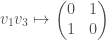


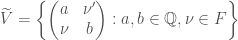
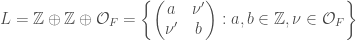
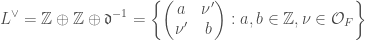


 where
where  is a morphism from
  satisfying the condition that
  .
.
 , and
, and  . Kahler manifolds which have complex structures with this behavior are called hyperkahler manifolds. Once again this is an important aspect that allows one to apply mirror symmetry to the geometric Langlands correspondence.
 -valued
  and therefore the moduli space of rank
  which is also the cotangent bundle
  of
of  :
: 
 ; in turn, the latter is the abelianization of the fundamental group
 , and we may think of
  . Combining this with the Corlette-Simpson correspondence between Higgs bundles and local systems (and hence representations of
 ). Cohomology with integral coefficients holds some information that gets lost when passing to rational coefficients; for instance, all the information about the torsion is lost. If we want to relate, say, torsion subgroups of different cohomologies to each other, we would need some sort of integral p-adic Hodge theory. In this post, we will discuss one approach to integral p-adic Hodge theory, called prismatic cohomology, developed by Bhargav Bhatt and Peter Scholze.
 -rings. A
  called a p-derivation, satisfying the following properties:

 consisting of a
  , such that
  -complete (this means that for every
  we have, considering
  and
and  ) and
) and  .
.![A=\mathbb{Z}_{p}[[u]]](https://s0.wp.com/latex.php?latex=A%3D%5Cmathbb%7BZ%7D_%7Bp%7D%5B%5Bu%5D%5D&bg=ffffff&fg=444444&s=0&c=20201002) and taking
and taking  . Another important example that we will show up again later in this post is given by
  and
and  , where
  is the canonical map (see also
  is an perfectoid ring. In fact, there is an equivalence of categories between perfect prisms and perfectoid rings, and one can go the other way via the
  construction, i.e. given a perfectoid ring
  , and there is a canonical map
  , and we set
  ; then the pair
  , is the category of prisms
  over
over  over
over  . We have functors
  and
and  which send
  , to be
  . As an example, in the special case that
  , then the prismatic cohomology
  in
in  -modules instead), prismatic F-crystals (prismatic crystals
 ![\phi^{*}\mathcal{E}[1/I]\to\mathcal{E}[1/I]](https://s0.wp.com/latex.php?latex=%5Cphi%5E%7B%2A%7D%5Cmathcal%7BE%7D%5B1%2FI%5D%5Cto%5Cmathcal%7BE%7D%5B1%2FI%5D&bg=ffffff&fg=444444&s=0&c=20201002) ), and notions of crystals where instead of modules we consider complexes (perfect or
), and notions of crystals where instead of modules we consider complexes (perfect or  , which corresponds to the Tate twist in etale cohomology. The prismatic cohomology also comes with a filtration, called the Nygaard filtration. These structures are important for some of the applications of prismatic cohomology. For instance, the two notions just discussed allows us to give a definition of syntomic cohomology as follows:
 that computes the de Rham cohomology of
  is related to
  as follows:
 (we call such an element
 ![\displaystyle R\Gamma_{\mathrm{et}}(\mathrm{Spec}(R)[1/p],\mathbb{Z}/p^{n})\cong (\Delta_{R/A}[1/d]/p^{n})^{\phi=1}](https://s0.wp.com/latex.php?latex=%5Cdisplaystyle+R%5CGamma_%7B%5Cmathrm%7Bet%7D%7D%28%5Cmathrm%7BSpec%7D%28R%29%5B1%2Fp%5D%2C%5Cmathbb%7BZ%7D%2Fp%5E%7Bn%7D%29%5Ccong+%28%5CDelta_%7BR%2FA%7D%5B1%2Fd%5D%2Fp%5E%7Bn%7D%29%5E%7B%5Cphi%3D1%7D&bg=ffffff&fg=444444&s=0&c=20201002)
 . Let
. Let  by gluing together the different
  , and then use the comparison theorems previously mentioned to prove the following result:
 which is perfectoid, and such that for any other perfectoid ring
  . As we just stated, a way to construct the perfectoidization is given by the perfected prismatic cohomology. Let
 . The pair
  is a perfect prism, and the quotient
  is a perfectoidization of
  ).
). be an etale morphism. We may express this as the composition
  , where
  is finite. We may express
  and
and  . Then we can define
 to
to  may be taken to be a Riemann-Hilbert functor, agreeing with previous constructions of Bhatt and Lurie. Inspired by this, in the more general case we can define
 is an
is an  . For an etale morphism
  be the sheaf
  on
on  , where
  is the constant sheaf of
 ![R=\mathbb{Z}[x_{1},\ldots,x_{n}]](https://s0.wp.com/latex.php?latex=R%3D%5Cmathbb%7BZ%7D%5Bx_%7B1%7D%2C%5Cldots%2Cx_%7Bn%7D%5D&bg=ffffff&fg=444444&s=0&c=20201002) . Let
. Let  is a zero divisor of
  A “global” version of this theorem is mixed-characteristic Kodaira vanishing up to finite covers, also proved by Bhatt, and which has applications to the minimal model program in birational geometry.
 of a p-adic formal scheme
  of
of  ). The prismatization
  , the Nygaard filtered prismatization of
  called the syntomification of
  , upon inverting
  , and let
  . Their respective groups of isometries are the unitary groups
  and
and  . These two groups form an example of a reductive dual pair. The theory of the local theta correspondence relates representations of one of these groups to representations of the other.
 can be viewed as a vector space over
  . We have a map
 has a cover called the metaplectic group; we will describe it in more detail shortly, but we say now that the importance of it for our purposes is that it has a special representation called the Weil representation, which as we shall shortly see will be useful in relating representations of
  . Its elements are given by
  , and we give it the group structure
 the Heisenberg group has a unique irreducible representation
  with central character
  is a Lagrangian decomposition, we can realize the representation
  (defined to be the subgroup
  of
of  ) and then define
 for
for  and
and  . We can compose this action with the representation
  of
of  . Now since the action of
  and
and  , we have a linear transformation
  of the underlying vector space
  of the representation
 . Since
  to be unitary, and so the action becomes well-defined up to
  . All in all, this means that we have a representation
 by the map
  , we get a map
  , where the group
  is an
is an  to the semidirect product
  . This representation of
  . If we could lift this to a map
  , then we could obtain a representation of
  by restricting the Weil representation
  to
to  of characters of
  satisfying certain conditions. Once we have this lifting, we denote the resulting representation of
  .
. from
from  , where
  is a representation of
  called the big theta lift of
  , and is called the small theta lift of
  be the completion of
  and
and  , as in the local case, and consider the tensor product
  . We have localizations
  for every
  . We want to put each of these together for every
  . “Restricted” means that all but finitely many of the factors in this product belong to the hyperspecial maximal compact subgroup
  of
of  , which is also a compact open subgroup of
  as a central subgroup. Now if we quotient out the restricted product
  such that
  , the resulting quotient is the “adelic” metaplectic group
  that we are looking for.
 of
of  is a Lagrangian decomposition, we have seen that we can realize the local Weil representation
  on
on  , the vector space of Schwarz functions of
  (the corresponding localization of
  , defined to be the restricted product
  .
. on the vector space
  , so-called because it is a generalization of the Jacobi theta function discussed in
  :
:
 of
of  to
to  to
to  , which means that we can consider
  on
on ![\displaystyle \theta(\varphi,f)(g)=\int_{[\mathrm{U}(V)]}\theta(\varphi)(g,h)\cdot \overline{f(h)}dh](https://s0.wp.com/latex.php?latex=%5Cdisplaystyle+%5Ctheta%28%5Cvarphi%2Cf%29%28g%29%3D%5Cint_%7B%5B%5Cmathrm%7BU%7D%28V%29%5D%7D%5Ctheta%28%5Cvarphi%29%28g%2Ch%29%5Ccdot+%5Coverline%7Bf%28h%29%7Ddh&bg=ffffff&fg=444444&s=0&c=20201002)
 when
when  . Meanwhile
  cannot be written as the sum of two squares; since squares are positive, we only need look at the numbers less than
  , we can see that it can once again be written as the sum of two squares,
  .
.


 to write a number
  or
or  ). If the
  on the upper half-plane called the theta function, defined as follows:
 . Re-indexing the summation we can also write the theta function as
 , and character
  (see also
  is a holomorphic function on the upper half-plane, bounded as the imaginary part of
 is an element of
  integer matrices with determinant
  if
if  “, but we will avoid this terminology in this post to keep things less confusing.)
 ) the above equation becomes
 and
and  such that
  . In other words, the coefficient
  counts how many pairs
  there are such that
  we mentioned earlier that tells us how many ways there are to write
  and this will tell us about sums of four squares. More precisely, the
  that tells us how many ways there are to write
 . Specializing to when
  , which is
  when
when 
 (here the symbol
  denotes the sum of the positive divisors of

 called strata, such that the closure of any stratum is a union of strata.
 to any stratum
  to
to  as the category whose objects are the cochain complexes in
  where the objects are the cochain complexes in
  (this is used if there is some stratification of
  ).
). ,
,  ,
,  ,
,  ,
,  , and
, and  , the first four being the derived functors corresponding to the usual operations of Hom, tensor product, pushforward, and pullback, respectively, and the last two are the derived “shriek” functors (see also
  be an algebraic variety with its stratification, and for every stratum
  denote its dimension. We write
  for the subcategory of
  whose cohomology sheaves are locally constant, and for any object
  of some derived category we write
  for its

 be the inclusion of a stratum

 , as the heart of this t-structure.
 , and let
 ![\mathcal{O}=k[[t]]](https://s0.wp.com/latex.php?latex=%5Cmathcal%7BO%7D%3Dk%5B%5Bt%5D%5D&bg=ffffff&fg=444444&s=0&c=20201002) . Let
. Let  and the positive loop group
  is defined to be the scheme whose
  . The affine Grassmannian is then defined to be the quotient
  .
. on the affine Grassmannian
  and the category
  of representations of the Langlands dual group
  of
of  which is adic with respect to a finitely generated ideal of definition
  , and the ideal of definition
  .
. , with the p-adic topology, with the ring of definition
  , and the ideal of definition
  .
. over some field
 ![A_{0}=k[[x]]](https://s0.wp.com/latex.php?latex=A_%7B0%7D%3Dk%5B%5Bx%5D%5D&bg=ffffff&fg=444444&s=0&c=20201002) , and the ideal of definition
, and the ideal of definition  .
. and ideal of definition
  for some
  .
.  . Any element of the ring of definition will always be power bounded.
 . Its set of power bounded elements is given by
  . Now let
 ![A=K^{\circ}[[T_{1},\ldots, T_{n}]]](https://s0.wp.com/latex.php?latex=A%3DK%5E%7B%5Ccirc%7D%5B%5BT_%7B1%7D%2C%5Cldots%2C+T_%7Bn%7D%5D%5D&bg=ffffff&fg=444444&s=0&c=20201002) with the
with the  . Then
  , and
, and  (see also
  . Then
  and ideal of definition given by
  .
. of a Huber ring
  consisting of a Huber ring
  .
. . They will form the basic building blocks of adic spaces, like affine schemes are to schemes or affinoid rigid analytic spaces are to rigid analytic spaces. We will proceed in the usual manner; first we define the underlying set, then we put a topology on it, and then construct a structure sheaf – except that in the case of adic spaces, what we will construct is merely a structure presheaf and may not always be a sheaf! Then we will define more general adic spaces to be something that locally looks like the adic spectrum of some Huber pair.
 on
on  whenever
  is in
is in  instead of
  , to drive home the idea that these (equivalence classes of) continuous valuations are the points of our space, on which elements of our ring
 .
.
 . If
. If  such that the map
  factors through
  where
where  where the limit is taken over all inclusions of rational subsets
  , and
, and  is similarly defined.
 , and for each point
  , such that it admits a covering of
  instead of
  . Let us now look at some examples of adic spaces.
 (which by the previous paragraph we may also simply write as
  , since
  is the set of power-bounded elements of
  (which by the same idea as above we may write as
  ). The underlying topological space of
  , also known as the adic closed unit disc. We can compare this with the closed unit disc discussed in
  . But every such maximal ideal gives rise to a continuous valuation on
  , where
  is such that
  for all real numbers
  in this order. Define a continuous valuation
  on
on 
 of the adic closed unit disc. This valuation sees
  , but
, but  for all
  and
and  will not miss the point
 ![\mathrm{Spa}(\mathbb{Z}_{p}[[ T]],\mathbb{Z}_{p}[[T]])](https://s0.wp.com/latex.php?latex=%5Cmathrm%7BSpa%7D%28%5Cmathbb%7BZ%7D_%7Bp%7D%5B%5B+T%5D%5D%2C%5Cmathbb%7BZ%7D_%7Bp%7D%5B%5BT%5D%5D%29&bg=ffffff&fg=444444&s=0&c=20201002) . This is the adic open unit disc. This has a map to
. This is the adic open unit disc. This has a map to  converges to
  in
in  is an isomorphism, then we say that
  -algebras, where
  may be thought of as a completed inverse limit
  , where each
  is an etale map. An example of a pro-etale cover is as follows. If we let
  (this is somewhat similar to the example involved in the Fontaine-Wintenberger theorem in
  is a pro-etale cover of
  of
of  , then for all
 (this is the cohomology of the sheaf of functions bounded by
  of a real Lie group
  , where
 ![\mathrm{SL}_{2}(\mathbb{Z}[i])](https://s0.wp.com/latex.php?latex=%5Cmathrm%7BSL%7D_%7B2%7D%28%5Cmathbb%7BZ%7D%5Bi%5D%29&bg=ffffff&fg=444444&s=0&c=20201002) (or we can also replace
(or we can also replace ![\mathbb{Z}[i]](https://s0.wp.com/latex.php?latex=%5Cmathbb%7BZ%7D%5Bi%5D&bg=ffffff&fg=444444&s=0&c=20201002) with the ring of integers of some other imaginary quadratic field). The groups involve look complex, but the theory of algebraic groups and in particular the method of Weil restriction allows us to look at them as real Lie groups. This is not an algebraic variety (one way to see this is that
with the ring of integers of some other imaginary quadratic field). The groups involve look complex, but the theory of algebraic groups and in particular the method of Weil restriction allows us to look at them as real Lie groups. This is not an algebraic variety (one way to see this is that  is hyperbolic 3-space, so a Bianchi manifold has 3 real dimensions and as such cannot be related to an algebraic variety the way a complex manifold can).
 for
for  . Meanwhile, we say that a Weil-Deligne representation (see also
  , and the monodromy operator
  is zero. Let us note that an unramified Weil-Deligne representation is determined by where the Frobenius element (which maps to
  gets sent to, up to conjugacy. Hence the unramified Weil-Deligne representations are in bijection with conjugacy classes of diagonalizable elements in
  .
. is the algebra of compactly supported locally constant functions on
  and
and  of the spherical Hecke algebra, their “product” is given by
 .
. .
. be the set of all cocharacters of
 ![\mathbb{C}[X_{\bullet}(T)]](https://s0.wp.com/latex.php?latex=%5Cmathbb%7BC%7D%5BX_%7B%5Cbullet%7D%28T%29%5D&bg=ffffff&fg=444444&s=0&c=20201002) be the ring formed by adjoining the elements of
be the ring formed by adjoining the elements of ![\mathbb{C}[X_{\bullet}(T)]^{W}](https://s0.wp.com/latex.php?latex=%5Cmathbb%7BC%7D%5BX_%7B%5Cbullet%7D%28T%29%5D%5E%7BW%7D&bg=ffffff&fg=444444&s=0&c=20201002) .
.![\displaystyle \mathcal{H}(\mathrm{GL}_{n}(F),\mathrm{GL}_{n}(\mathcal{O}_{F}))\cong \mathbb{C}[X_{\bullet}(T)]^{W}](https://s0.wp.com/latex.php?latex=%5Cdisplaystyle+%5Cmathcal%7BH%7D%28%5Cmathrm%7BGL%7D_%7Bn%7D%28F%29%2C%5Cmathrm%7BGL%7D_%7Bn%7D%28%5Cmathcal%7BO%7D_%7BF%7D%29%29%5Ccong+%5Cmathbb%7BC%7D%5BX_%7B%5Cbullet%7D%28T%29%5D%5E%7BW%7D&bg=ffffff&fg=444444&s=0&c=20201002) .
. to be
to be ![\mathrm{Spec}(\mathbb{C}[X_{\bullet}(T)])](https://s0.wp.com/latex.php?latex=%5Cmathrm%7BSpec%7D%28%5Cmathbb%7BC%7D%5BX_%7B%5Cbullet%7D%28T%29%5D%29&bg=ffffff&fg=444444&s=0&c=20201002) . Then homomorphisms
. Then homomorphisms ![\mathbb{C}[X_{\bullet}(T)]^{W}\to\mathbb{C}](https://s0.wp.com/latex.php?latex=%5Cmathbb%7BC%7D%5BX_%7B%5Cbullet%7D%28T%29%5D%5E%7BW%7D%5Cto%5Cmathbb%7BC%7D&bg=ffffff&fg=444444&s=0&c=20201002) correspond to
correspond to  . These conjugacy classes, in turn, are in bijection with the conjugacy classes of diagonalizable elements in