June | 2023 | Theories and Theorems

Hilbert Modular Surfaces and Hilbert Modular Forms: The Basics

A Hilbert modular surface is a kind of Shimura variety (see Shimura Varieties), in a sense one of the next simplest after modular curves (although Shimura curves have lower dimension and Siegel modular threefolds have a simpler moduli interpretation). Aside from being a higher-dimensional analogue of modular curves, Hilbert modular surfaces possess interesting structure not present in modular curves. For example, Hilbert modular forms may contain embedded modular curves as codimension $1$ subvarieties!

We begin with the definition. Let $F=\mathbb{Q}(\sqrt{d})$ , where $d$ is a squarefree positive integer, i.e. $F$ is a real quadratic field. We denote its ring of integers by $\mathcal{O}_{F}$ . The group $\Gamma=\mathrm{SL}_{2}(\mathcal{O}_{F})$ acts on the product $\mathbb{H}\times \mathbb{H}$ of two upper half-planes as follows:

$\displaystyle \begin{pmatrix} a & b \\ c & d \end{pmatrix}(z_{1},z_{2})=\left(\frac{az_{1}+b}{cz_{1}+d},\frac{a'z_{2}+b'}{c'z_{2}+d'}\right)$

for $(z_{1},z_{2})\in \mathbb{H}\times\mathbb{H}$ , where $a',b',c',d'$ are the Galois conjugates of $a,b,c,d$ . If we then take the left quotient of $\mathbb{H}\times\mathbb{H}$ by this action of $\Gamma)$ , we then end up with a complex analytic surface $Y(\Gamma)$ , which is non-compact. Just as the “open” modular curve constructed in The Moduli Space of Elliptic Curves parametrizes elliptic curves over $\mathbb{C}$ , the open modular surface $Y(\Gamma)$ which we have just constructed parametrizes abelian surfaces $A$ over $\mathbb{C}$ with an extra “real multiplication” structure, which is an embedding of $\mathcal{O}_{F}$ into their ring of endomorphisms $\mathrm{End}(A)$ .

We may “compactify” the above construction by instead considering the quotient $\Gamma\backslash(\mathbb{H}\times\mathbb{H}\cup\mathbb{P}^1(F))$ (note that $\mathbb{P}^{1}(F)$ is also equipped with an action of $\Gamma$ ), which adds a finite number (equal to the class number of $F$ ) of points called cusps. This compactification, which we denote $X(\Gamma)$ , will be singular. However, by the theory developed by Heisuke Hironaka, there is a way to “resolve” the singularities, and by applying this theory we may obtain a smooth projective surface $\widetilde{X}(\Gamma)$ .

Hilbert modular surfaces are the natural home of Hilbert modular forms (although Hilbert modular forms live on Hilbert modular varieties, more generally, as we mention in the next paragraph). A Hilbert modular form of weight $(k_{1},k_{2})$ is a meromorphic function $f$ on $\mathbb{H}\times\mathbb{H}$ such that, for $\gamma=\begin{pmatrix}a & b \\ c & d\end{pmatrix}\in\Gamma$ , we have

$\displaystyle f(\gamma z)=(cz_{1}+d)^{k_{1}}(c'z_{2}+d')^{k_{2}}f(z_{1},z_{2})$

From the point of view of algebraic geometry, Hilbert modular forms can also be obtained as sections of certain sheaves on a Hilbert modular surface.

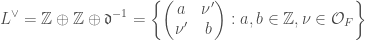
Before we continue our discussion of Hilbert modular surfaces, we note that all of the above constructions may be generalized by letting $F$ be a more general totally real field, instead of just a real quadratic field. This leads to the more general notion of a Hilbert modular variety, and of more general Hilbert modular forms. We also note that instead of $\Gamma=\mathrm{SL}_{2}(\mathcal{O}_{F})$ , we could instead consider some nontrivial level structure $\Gamma=\Gamma(\mathcal{O}_{F}\oplus\mathfrak{a})$ , where $\mathfrak{a}$ is some fractional ideal of $\mathcal{O}_{F}$ . The group $\Gamma(\mathcal{O}_{F}\oplus\mathfrak{a})$ is defined to be the group of matrices of the form $\begin{pmatrix} a & b \\ c & d \end{pmatrix}$ where $a,d\in\mathcal{O}_{F}$ , $b\in\mathfrak{a}^{-1}$ , and $c\in\mathfrak{a}$ .

A Whirlwind Introduction to Clifford Algebras and Spin Groups

We have so far described Hilbert modular surfaces and Hilbert modular forms in terms of the group $\mathrm{SL}_{2}(F)$ . However there is another way to describe them via the exceptional isomorphisms of spin groups (which are double covers of special orthogonal groups, see also Rotations in Three Dimensions) with other groups – In our case, we have the isomorphism $\mathrm{Spin}(2,2)\simeq\mathrm{SL}_{2}(F)$ . Let us discuss first the general theory behind spin groups of signature $(2,n)$ and their associated symmetric spaces, and then later we apply it to the specific case of Hilbert modular surfaces.

Let $(V,q)$ be a pair consisting of a vector space $V$ over $\mathbb{Q}$ and a quadratic form $q$ . The orthogonal group $\mathrm{O}(V)$ is the subgroup of the group of linear transformations of $V$ which preserve $q$ . The Clifford algebra $C_{V}$ associated to $(V,q)$ is the quotient of the tensor algebra of $V$ by the relation, for all $v\in V$ ,

$\displaystyle v^{2}=q(v)$

The Clifford algebra generalizes many familiar constructions such as the complex numbers (for $V=\mathbb{R}$ and $q(v)=-v^{2}$ ) and Hamilton’s quaternions for $V=\mathbb{R}^{2}$ and $q(v_{1}+v_{2})=-v_{1}^{2}-v_{2}^{2}$ . Note that, unlike the complex numbers, more general Clifford algebras such as Hamilton’s quaternions have more than one type of “conjugation”. The first, which we shall call $J$ , is induced by negation of basis elements of $V$ . Another is given by cyclically permuting the tensor factors of an element so that $x^{t}=v_{2}\otimes\ldots \otimes v_{m}\otimes v_{1}$ for $v=v_{1}\otimes\ldots\otimes v_{m}$ . This second conjugation allows us to define the Clifford norm:

$\displaystyle \mathrm{Nm}(v)=v^{t}v$

The even Clifford algebra $C_{V}^{0}$ of $C_{V}$ is the subalgebra generated by elements which are a product of an even number of basis elements of $V$ . The odd part $C_{V}^{1}$ is similarly defined, and we have the decomposition $C_{V}=C_{V}^{0}\oplus C_{V}^{1}$ . The Clifford group is defined to be the set of all invertible elements $v$ of the Clifford algebra such that $vVJ(v)^{-1}=V$ . The intersection of the even Clifford algebra and the Clifford group is called $\mathrm{GSpin}(V)$ . The set of elements of $\mathrm{GSpin}(V)$ whose Clifford norm is equal to $1$ is called $\mathrm{Spin}(V)$ .

We now mention some facts about the special case when $V$ has dimension $4$ that we will use later when we discuss Hilbert modular surfaces again. Let $v_{1},v_{2},v_{3},v_{4}$ be a basis of $V$ such that $q(v_{i})\neq 0$ for all $i$ . Let $\delta=v_{1}v_{2}v_{3}v_{4}$ . The center $Z$ of the Clifford algebra associated to $(V,q)$ is then isomorphic to $\mathbb{Q}+\mathbb{Q}\delta$ , and the even Clifford algebra admits the description

$\displaystyle C_{V}^{0}=Z+Zv_{1}v_{2}+Zv_{2}v_{3}+Zv_{1}v_{3}$

Fix an element $v_{0}\in V$ such that $q(v_{0})\neq 0$ and for $v\in C_{V}^{0}$ let $v^{\sigma}=v_{0}vv_{0}^{-1}$ . We define the new vector space $\widetilde{V}$ to be the set of all elements $v$ of $C_{V}^{0}$ such that the automorphism $v^{\sigma}$ agrees with the conjugation $v^{t}$ , and we equip $\widetilde{V}$ with the quadratic form $\widetilde{q}(v)=q(v_{0})\cdot \mathrm{Nm}(v)$ . 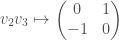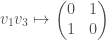It turns out that $(\widetilde{V},\widetilde{q})$ is isometric to $(V,q)$ , and the upshot is that we can now describe the action of an element $g\in\mathrm{Spin}(V)$ on an element $v\in\widetilde{V}$ as follows:

$\displaystyle g(v)=gVg^{-\sigma}$ .

Symmetric Spaces for Orthogonal Groups of Signature (2,n): Three Descriptions

The upper-half plane is the “symmetric space” for the group $\mathrm{SL}_{2}(\mathbb{R})$ , and may be obtained as the quotient of $\mathrm{SL}_{2}(\mathbb{R})$ by its locally compact subgroup $\mathrm{SO}(2)$ . We want to generalize this to the group $\mathrm{O}(V)$ , but it is often useful to have different descriptions of the symmetric space. We will discuss three different descriptions of the symmetric space on which $\mathrm{O}(V)$ acts, each one with its own advantages and disadvantages.

First we give the “Grassmannian model“. The Grassmannian parametrizes $k$ -dimensional subspaces of a vector space. It is a generalization of projective space (which is the special case when $k=1$ ). In our case, we want to parametrize $2$ -dimensional spaces of $V$ , with the additional condition that the quadratic form $q$ is positive definite on this space:

$\displaystyle \mathrm{Gr}(V)=\lbrace v\in V:\mathrm{dim}(v)=2\mbox{ and }q\vert_{v}>0\rbrace$

The group $\mathrm{O}(V)$ acts on $\mathrm{Gr}(V)$ , and the stabilizer of an element $v_{0}$ is a maximal compact subgroup $K$ , which is isomorphic to $\mathrm{O}(2)\times \mathrm{O}(n)$ . Therefore we can see that $\mathrm{Gr}(V)\cong \mathrm{O}(V)/K$ , and provides a realization of its associated symmetric space. However, in this model it is harder to see the complex analytic structure.

This problem can be remedied by considering the “projective model“. Let $V(\mathbb{C})$ be the complexification of $V$ and define

$\displaystyle \mathcal{K}=\lbrace[z]\in\mathbb{P}(V(\mathbb{C})):(z,z)=0,(z,\overline{z})>0\rbrace$

Now $\mathcal{K}$ is an $n$ -dimensional complex manifold consisting of two connected components. We choose one of these components and denote it by $\mathcal{K}^{+}$ – this is our symmetric space. Although the complex analytic structure is easier to see in the projective model, it is hard to relate this model to well-known examples of symmetric spaces such as the upper half-plane (which is the case when $n=1$ ).

Finally we consider the “tube domain model“. Let $e_{1}$ be a nonzero isotropic vector in $V$ and let $e_{2}$ be another vector in $V$ such that $(e_{1},e_{2})=1$ . We let $W$ be the intersection of the orthogonal complements of $e_{1}$ and $e_{2}$ in $V$ , so that

$\displaystyle V=W\oplus \mathbb{C}e_{1}\oplus\mathbb{C}e_{2}$

On the vector space $W$ , the restriction of the quadratic form $q$ has signature $1,n-1$ . We let $W(\mathbb{C})$ denote the complexification of $W$ and define

$\displaystyle \mathcal{H}=\lbrace z\in W(\mathbb{C}):q(\mathrm{Im}(z))>0)\rbrace$

We can define a biholomorphic map between $\mathcal{H}$ and $\mathcal{K}$ by sending $z$ to $[(z,1,-q(z)-q(e_{2}))]$ . We denote the preimage of $\mathcal{K}^{+}$ by $\mathcal{H}^{+}$ – the latter is analogous to the upper half-plane.

Heegner Divisors

Let us now consider smaller modular varieties embedded in other bigger modular varieties. Let $L$ be a lattice in $V$ . The idea is that if we pick a vector $\lambda$ in the dual lattice $L^{\vee}$ in $V$ , and consider the orthogonal complement of $\lambda$ in $V$ , what we get is actually a vector space of signature $2,n-1$ , to which we can once again apply the preceding constructions! Applied to the case of Hilbert modular surfaces, this explains the embedded modular curves. In symbols, we have

$\displaystyle H_{\lambda}=\lbrace [Z]\in\mathcal{K}^{+}:(Z,\lambda)=0\rbrace$

If we write $\lambda=\lambda_{W}+ae_{2}+be_{1}$ , then we can also describe $H_{\lambda}$ in the tube domain model as follows:

$\displaystyle H_{\lambda}=\lbrace z\in\mathcal{H}^{+}:aq(z)-(z,\lambda_{W})-aq(e_{2})-b=0\rbrace$

We can now define the Heegner divisor $H(\beta,m)$ as the sum of all the $H_{\lambda}$ where $\lambda\in\beta+L$ satisfies the condition that $q(\lambda)=m$ . We can further define the composite Heegner divisor $H(m)$ as half the sum of all Heegner divisors $H(\beta,m)$ as $\beta$ runs over $L^{\vee}/L$ .

Back to Hilbert Modular Surfaces

We now go back to our setting of Hilbert modular surfaces and apply the above theory to the $4$ -dimensional vector space $V=\mathbb{Q}\oplus\mathbb{Q}\oplus F$ , equipped with the quadratic form $q(a,b,\nu)=\nu\nu'-ab$ . We choose the following basis for $V$ :

$\displaystyle v_{1}=(1,1,0)$

$\displaystyle v_{2}=(1,-1,0)$

$\displaystyle v_{3}=(0,0,1)$

$\displaystyle v_{4}=(0,0,\sqrt{d})$

In this case the center of the Clifford algebra is isomorphic to $F$ , and the even Clifford algebra $C_{V}^{0}$ of $V$ is of the form $C_{V}^{0}=F+Fv_{1}v_{2}+Fv_{2}v_{3}+Fv_{1}v_{3}$ . Via the assignments

$\displaystyle 1\mapsto\begin{pmatrix}1 & 0 \\ 0 & 1\end{pmatrix}$

$\displaystyle v_{1}v_{2}\mapsto\begin{pmatrix}1 & 0 \\ 0 & -1\end{pmatrix}$

$\displaystyle v_{2}v_{3}\mapsto\begin{pmatrix}0 & 1 \\ -1 & 0\end{pmatrix}$

$\displaystyle v_{1}v_{3}\mapsto\begin{pmatrix}0 & 1 \\ 1 & 0\end{pmatrix}$

we have an isomorphism between $C_{V}^{0}$ and $M_{2}(F)$ . Furthermore, the Clifford norm on $C_{V}^{0}$ corresponds to the determinant on $M_{2}(F)$ . All in all, this gives us an isomorphism between $\mathrm{Spin}_{V}$ and $\mathrm{SL}_{2}(F)$ . The theory we have discussed earlier provides us with the following vector space $\widetilde{V}$ isomorphic to $V$ :

$\displaystyle \widetilde{V}=\left\lbrace \begin{pmatrix} a & \nu' \\ \nu & b\end{pmatrix}:a,b\in\mathbb{Q},\nu\in F\right\rbrace$

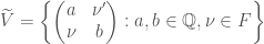
We also have a description of the lattices $L$ and $L^{\vee}$ as matrices inside $\widetilde{V}$ as follows:

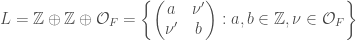
$\displaystyle L=\mathbb{Z}\oplus\mathbb{Z}\oplus\mathcal{O}_{F}=\left\lbrace\begin{pmatrix}a & \nu' \\ \nu' & b\end{pmatrix}:a,b\in\mathbb{Z},\nu\in\mathcal{O}_{F}\right\rbrace$

$\displaystyle L^{\vee}=\mathbb{Z}\oplus\mathbb{Z}\oplus\mathfrak{d}^{-1}=\left\lbrace\begin{pmatrix}a & \nu' \\ \nu' & b\end{pmatrix}:a,b\in\mathbb{Z},\nu\in\mathcal{O}_{F}\right\rbrace$

It turns out, just as we have 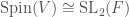$\mathrm{Spin}(V)\cong \mathrm{SL}_{2}(F)$ , we also have 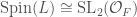$\mathrm{Spin}(L)\cong\mathrm{SL}_{2}(\mathcal{O}_{F})$ . In turn this gives us an isomorphism $Y(\Gamma)\cong Y(\mathrm{Spin}(L))$ .

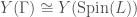Now we apply the general theory of Heegner divisors. In the special case of Hilbert modular surfaces, the Heegner divisors $H(-m/D)$ where $D$ is the discriminant of $F$ are also known as Hirzebruch-Zagier divisors. They have the explicit description

$\displaystyle T_{m}=\sum\lbrace(z_{1},z_{2}\in\mathbb{H}\times\mathbb{H}):az_{1}z_{2}+\lambda z_{1}+\lambda' z_{2}+b\rbrace$

where the sum is over all $(a,b,\lambda)\in L^{\vee}/\lbrace\pm 1\rbrace$ such that $ab-\lambda\lambda'=m$ . As a special case, $T_{1}$ is the modular curve of level $1$ (i.e. the compactified moduli space of elliptic curves).

Borcherds Products and the Kudla Program: A Preview

Hirzebruch-Zagier divisors are related to certain Hilbert modular forms called Borcherds products, which arise as “theta lifts” (see also The Theta Correspondence) of weakly holomorphic modular forms (which are almost the same as modular forms, but the holomorphicity condition at the cusps is relaxed). Here “theta lifts” is in quotes because the liftings are somewhat different from what is described in The Theta Correspondence; for one, the integral is divergent and requires a “regularization” to get it to converge, and the lifting is multiplicative, which gives it an expression as an infinite product – hence the name “Borcherds products”.

The Hirzebruch-Zagier divisors, or more generally the Heegner divisors, or even more generally “special cycles” can also be put together in a certain way to form a generating series, which should form a “modular form valued in the Chow group”. This is part of what is known as the “Kudla program” which has applications for instance to conjectures on special values of L-functions (which generalize the Birch and Swinnerton-Dyer conjecture). These and other fascinating aspects of orthogonal and unitary Shimura varieties will hopefully be covered in future posts.

References:

Hilbert modular variety on Wikipedia

Hilbert modular form on Wikipedia

Hilbert modular forms and their applications by Jan Hendrik Bruinier

Hilbert Modular Surfaces by Gerard van der Geer

The 1-2-3 of Modular Forms by Jan Hendrik Bruinier, Gunter Harder, Gerard van der Geer, and Don Zagier

Theories and Theorems

Math and Physics for Everyone

Month: June 2023

Hilbert Modular Surfaces