complex analysis

A Hecke operator is a certain kind of linear transformation on the space of modular forms or cusp forms (see also Modular Forms) of a certain fixed weight $k$ . They were originally used (and now named after) Erich Hecke, who used them to study L-functions (see also Zeta Functions and L-Functions) and in particular to determine the conditions for whether an L-series $\sum_{n=1}^{\infty}a_{n}n^{-s}$ has an Euler product. Together with the meromorphic continuation and the functional equation, these are the important properties of the Riemann zeta function, which L-functions are supposed to be generalizations of. Hecke’s study was inspired by the work of Bernhard Riemann on the zeta function.

An example of a Hecke operator is the one commonly denoted $T_{p}$ , for $p$ a prime number. To understand it conceptually, we must take the view of modular forms as functions on lattices. This is equivalent to the definition of modular forms as functions on the upper half-plane, if we recall that a lattice $\Lambda$ can also be expressed as $\mathbb{Z}+\tau\mathbb{Z}$ where $\tau$ is a complex number in the upper half-plane (see also The Moduli Space of Elliptic Curves).

In this view a modular form is a function on the space of lattices on $\mathbb{C}$ such that

$f(\mathbb{Z}+\tau\mathbb{Z})$ is holomorphic as a function on the upper half-plane
$f(\mathbb{Z}+\tau\mathbb{Z})$ is bounded as $\tau$ goes to $i\infty$
$f(\mu\Lambda)=\mu^{-k}f(\Lambda)$ for some nonzero complex number $\mu$ , and $k$ is the weight of the modular form

Now we define the Hecke operator $T_{p}$ by what it does to a modular form $f(\Lambda)$ of weight $k$ as follows:

$\displaystyle T_{p}f(\Lambda)=p^{k-1}\sum_{\Lambda'\subset \Lambda}f(\Lambda')$

where $\Lambda'$ runs over the sublattices of $\Lambda$ of index $p$ . In other words, applying $T_{p}$ to a modular form gives back a modular form whose value on a lattice $\Lambda$ is the sum of the values of the original modular form on the sublattices of $\Lambda$ of index $p$ , times some factor that depends on the Hecke operator and the weight of the modular form.

Hecke operators are also often defined via their effect on the Fourier expansion of a modular form. Let $f(\tau)$ be a modular form of weight $k$ whose Fourier expansion is given by $\sum_{n=0}^{\infty}a_{i}q^{i}$ , where we have adopted the convention $q=e^{2\pi i \tau}$ which is common in the theory of modular forms (hence this Fourier expansion is also known as a $q$ -expansion). Then the effect of a Hecke operator $T_{p}$ is as follows:

$\displaystyle T_{p}f(\tau)=\sum_{n=0}^{\infty}(a_{pn}+p^{k-1}a_{n/p})q^{n}$

where $a_{n/p}=0$ when $p$ does not divide $n$ . To see why this follows from our first definition of the Hecke operator, we note that if our lattice is given by $\mathbb{Z}+\tau\mathbb{Z}$ , there are $p+1$ sublattices of index $p$ : There are $p$ of these sublattices given by $p\mathbb{Z}+(j+\tau)\mathbb{Z}$ for $j$ ranging from $0$ to $p-1$ , and another one given by $\mathbb{Z}+(p\tau)\mathbb{Z}$ . Let us split up the Hecke operators as follows:

$\displaystyle T_{p}f(\mathbb{Z}+\tau\mathbb{Z})=p^{k-1}\sum_{j=0}^{p-1}f(p\mathbb{Z}+(j+\tau)\mathbb{Z})+p^{k-1}f(\mathbb{Z}+p\tau\mathbb{Z})=\Sigma_{1}+\Sigma_{2}$

where $\Sigma_{1}=p^{k-1}\sum_{j=0}^{p-1}f(p\mathbb{Z}+(j+\tau)\mathbb{Z})$ and $\Sigma_{2}=p^{k-1}f(\mathbb{Z}+p\tau\mathbb{Z})$ . Let us focus on the former first. We have

$\displaystyle \Sigma_{1}=p^{k-1}\sum_{j=0}^{p-1}f(p\mathbb{Z}+(j+\tau)\mathbb{Z})$

But applying the third property of modular forms above, namely that $f(\mu\Lambda)=\mu^{-k}f(\Lambda)$ with $\mu=p$ , we have

$\displaystyle \Sigma_{1}=p^{-1}\sum_{j=0}^{p-1}f(\mathbb{Z}+((j+\tau)/p)\mathbb{Z})$

Now our argument inside the modular forms being summed are in the usual way we write them, except that instead of $\tau$ we have $((j+\tau)/p)$ , so we expand them as a Fourier series

$\displaystyle \Sigma_{1}=p^{-1}\sum_{j=0}^{p-1}\sum_{n=0}^{\infty}a_{n}e^{2\pi i n((j+\tau)/p)}$

We can switch the summations since one of them is finite

$\displaystyle \Sigma_{1}=p^{-1}\sum_{n=0}^{\infty}\sum_{j=0}^{p-1}a_{n}e^{2\pi i n((j+\tau)/p)}$

The inner sum over $j$ is zero unless $p$ divides $n$ , in which case the sum is equal to $p$ . This gives us

$\displaystyle \Sigma_{1}=p^{-1}\sum_{n=0}^{\infty}a_{pn}q^{n}$

where again $q=e^{2\pi i \tau}$ . Now consider $\Sigma_{2}$ . We have

$\displaystyle \Sigma_{2}=p^{k-1}f(\mathbb{Z}+p\tau\mathbb{Z})$

Expanding the right hand side into a Fourier series, we have

$\displaystyle \Sigma_{2}=p^{k-1}\sum_{n}a_{n}e^{2\pi i n p\tau}$

Reindexing, we have

$\displaystyle \Sigma_{2}=p^{k-1}\sum_{n}a_{n/p}q^{n}$

and adding together $\Sigma_{1}$ and $\Sigma_{2}$ gives us our result.

The Hecke operators can be defined not only for prime numbers, but for all natural numbers, and any two Hecke operators $T_{m}$ and $T_{n}$ commute with each other. They preserve the weight of a modular form, and take cusp forms to cusp forms (this can be seen via their effect on the Fourier series). We can also define Hecke operators for modular forms with level structure, but it is more complicated and has some subtleties when for the Hecke operator $T_{n}$ we have $n$ sharing a common factor with the level.

If a cusp form $f$ is an eigenvector for a Hecke operator $T_{n}$ , and it is normalized, i.e. its Fourier coefficient $a_{1}$ is equal to $1$ , then the corresponding eigenvalue of the Hecke operator $T_{n}$ on $f$ is precisely the Fourier coefficient $a_{n}$ .

Now the Hecke operators satisfy the following multiplicativity properties:

$T_{m}T_{n}=T_{mn}$ for $m$ and $n$ mutually prime
$T_{p^{n}}T_{p}=T_{p^{n+1}}+p^{k-1}T_{p}$ for $p$ prime

Suppose we have an L-series $\sum_{n}a_{n}n^{-s}$ . This L-series will have an Euler product if and only if the coefficients $a_{n}$ satisfy the following:

$a_{m}a_{n}=a_{mn}$ for $m$ and $n$ mutually prime
$a_{p^{n}}T_{p}=a_{p^{n+1}}+p^{k-1}a_{p}$ for $p$ prime

Given that the Fourier coefficients of a normalized Hecke eigenform (a normalized cusp form that is a simultaneous eigenvector for all the Hecke operators) are the eigenvalues of the Hecke operators, we see that the L-series of a normalized Hecke eigenform has an Euler product.

In addition to the Hecke operators $T_{n}$ , there are also other closely related operators such as the diamond operator $\langle n\rangle$ and another operator denoted $U_{p}$ . These and more on Hecke operators, such as other ways to define them with double coset operators or Hecke correspondences will hopefully be discussed in future posts.

References:

Hecke Operator on Wikipedia

Modular Forms by Andrew Snowden

Congruences between Modular Forms by Frank Calegari

A First Course in Modular Forms by Fred Diamond and Jerry Shurman

Advanced Topics in the Arithmetic of Elliptic Curves by Joseph H. Silverman

We have discussed a lot of mathematical topics on this blog, with some of them touching on rather advanced subjects. But aside from a few comments about holomorphic functions and meromorphic functions in The Moduli Space of Elliptic Curves, we have not yet discussed one of the most interesting subjects that every aspiring mathematician has to learn about, complex analysis.

Complex analysis refers to the study of functions of complex numbers, including properties of these functions related to concepts in calculus such as differentiation and integration (see An Intuitive Introduction to Calculus). Aside from being an interesting subject in itself, complex analysis is also related to many other areas of mathematics such as algebraic geometry and differential geometry.

But before we discuss functions of a complex variable, we will first review the concept of Taylor expansions from basic calculus. Consider a function $f(x)$ where $x$ is a real variable. If $f(x)$ is infinitely differentiable at $x=0$ , we can express it as a power series as follows:

$\displaystyle f(x)=f(0)+f'(0)x+\frac{f''(0)}{2!}x^{2}+\frac{f'''(0)}{3!}x^{3}+...$

where $f'(0)$ refers to the first derivative of $f(x)$ evaluated at $x=0$ , $f''(0)$ refers to the second derivative of $f(x)$ evaluated at $x=0$ , and so on. More generally, the $n$ -th coefficient of this power series is given by

$\displaystyle \frac{f^{(n)}(0)}{n!}$

where $f^{(n)}(0)$ refers to the $n$ -th derivative of $f(x)$ evaluated at $x=0$ . This is called the Taylor expansion (or Taylor series) of the function $f(x)$ around $x=0$ . For example, for the sine function, we have

$\displaystyle \text{sin}(x)=x-\frac{x^{3}}{3!}+\frac{x^{5}}{5!}-...$

More generally, if the function $f(x)$ is infinitely differentiable at $x=a$ , we can obtain the Taylor expansion of $f(x)$ around $x=a$ using the following formula:

$\displaystyle f(x-a)=f(a)+f'(a)(x-a)+\frac{f''(a)}{2!}(x-a)^{2}+\frac{f'''(a)}{3!}(x-a)^{3}+...$

If a function $f(x)$ can be expressed as a power series at every point of some interval $U$ in the real line, then we say that $f(x)$ is real analytic on $U$ .

Now we bring in complex numbers. Consider now a function $f(z)$ where $z$ is a complex variable. If $f(z)$ can be expressed as a power series at every point of an open disk (the set of all complex numbers $z$ such that the magnitude $|z-z_{0}|$ is less than $\delta$ for some complex number $z_{0}$ and some positive real number $\delta$ ) $U$ in the complex plane, then we say that $f(z)$ is complex analytic on $U$ . Since the rest of this post discusses functions of a complex variable, I will be using “analytic” to refer to “complex analytic”, as opposed to “real analytic”.

Now that we know what an analytic function is, we next discuss the concept of holomorphic functions. If $f(x)$ is a function of a real variable, we define its derivative at $x_{0}$ as follows:

$\displaystyle f'(x_{0})=\lim_{x\to x_{0}}\frac{f(x)-f(x_{0})}{x-x_{0}}$

If we have a complex function $f(z)$ , the definition is the same:

$\displaystyle f'(z_{0})=\lim_{z\to z_{0}}\frac{f(z)-f(z_{0})}{z-z_{0}}$

However, note that the value of $z$ can approach $z_{0}$ in many different ways! For example, let $f(z)=\bar{z}$ , i.e. $f(z)$ gives the complex conjugate of the complex variable $z$ . Let $z_{0}=0$ . Since $z=x+iy$ , we have $f(z)=\bar{z}=x-iy$ .

$\displaystyle f'(0)=\lim_{z\to 0}\frac{x-iy-0}{x+iy-0}$

$\displaystyle f'(0)=\lim_{z\to 0}\frac{x-iy}{x+iy}$

If, for example, $z$ is purely real, i.e. $y=0$ , then we have

$\displaystyle f'(0)=\lim_{z\to 0}\frac{x}{x}$

$\displaystyle f'(0)=1$

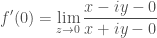
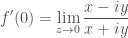
But if $z$ is purely imaginary, i.e. $x=0$ , then we have

$\displaystyle f'(0)=\lim_{z\to 0}\frac{-iy}{iy}$

$\displaystyle f'(0)=-1$

We see that the value of $f'(0)$ is different depending on how we approach the limit $z\to 0$ !

A function of complex numbers for which the derivative is the same regardless of how we take the limit $z\to z_{0}$ , for all $z_{0}$ in its domain, is called a holomorphic function. The function $f(z)=\bar{z}$ discussed above is not a holomorphic function on the complex plane, since the derivative is different depending on how we take the limit.

Now, it is known that a function of a complex number is holomorphic on a certain domain if and only if it is analytic in that same domain. Hence, the two terms are often used interchangeably, even though the concepts are defined differently. A function that is analytic (or holomorphic) on the entire complex plane is called an entire function.

If a function is analytic, then it must satisfy the Cauchy-Riemann equations (named after two pioneers of complex analysis, Augustin-Louis Cauchy and Bernhard Riemann). Let us elaborate on what these equations are a bit. Just as we can express a complex number $z$ as $x+iy$ , we can also express a function $f(z)$ of $z$ as $u(z)+iv(z)$ , or, going further and putting together these two expressions, as $u(x,y)+iv(x,y)$ . The Cauchy-Riemann equations are then given by

$\displaystyle \frac{\partial{u}}{\partial{x}}=\frac{\partial{v}}{\partial{y}}$

$\displaystyle \frac{\partial{u}}{\partial{y}}=-\frac{\partial{v}}{\partial{x}}$

Once again, if a function 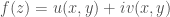$f(z)=u(x,y)+iv(x,y)$ is analytic, then it must satisfy the Cauchy-Riemann equations. Therefore, if it does not satisfy the Cauchy-Riemann equations, we know for sure that it is not analytic. But we should still be careful – just because a function satisfies the Cauchy-Riemann equations does not always mean that it is analytic! We also often say that satisfying the Cauchy-Riemann equations is a “necessary”, but not “sufficient” condition for a function of a complex number to be analytic.

Analytic functions have some very special properties. For instance, since we have already talked about differentiation, we may also now consider integration. Just as differentiation is more complicated in the complex plane than on the real line, because in the former there are different directions in which we may take the limit, integration is also more complicated on the complex plane as opposed to integration on the real line. When we perform integration over the variable $dz$ , we will usually specify a “contour”, or a “path” over which we integrate.

We may reasonably expect that the integral of a function will depend not only on the “starting point” and “endpoint”, as in the real case, but also on the choice of contour. However, if we have an analytic function defined on a simply connected (see Homotopy Theory) domain, and the contour is inside this domain, then the integral will not depend on the choice of contour! This has the consequence that if our contour is a loop, the integral of the analytic function will always be zero. This very important theorem in complex analysis is known as the Cauchy integral theorem. In symbols, we write

$\displaystyle \oint_{\gamma}f(z)dz=0$

where the symbol $\oint$ means that the contour of integration is a loop. The symbol $\gamma$ refers to the contour, i.e. it may be a circle, or some other kind of loop – usually whenever one sees this symbol the author will specify the contour that it refers to.

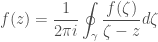
Another important result in complex integration is what is known as the Cauchy integral formula, which relates an analytic function to its values on the boundary of some disk contained in the domain of the function:

$\displaystyle f(z)=\frac{1}{2\pi i}\oint_{\gamma}\frac{f(\zeta)}{\zeta-z}d\zeta$

By taking the derivative of both sides with respect to $z$ , we obtain what is also known as the Cauchy differentiation formula:

$\displaystyle f'(z)=\frac{1}{2\pi i}\oint_{\gamma}\frac{f(\zeta)}{(\zeta-z)^{2}}d\zeta$

The reader may notice that on one side of this fascinating formula is a derivative, while on the other side there is an integral – in the words of the Wikipedia article on the Cauchy integral formula, in complex analysis, “differentiation is equivalent to integration”!

These theorems regarding integration lead to the residue theorem, a very powerful tool for calculating the contour integrals of meromorphic functions (see The Moduli Space of Elliptic Curves) – functions which would have been analytic in their domain, except that they have singularities of a certain kind (called poles) at certain points. A more detailed discussion of meromorphic functions, singularities and the residue theorem is left to the references for now.

Aside from these results, analytic functions also have many other interesting properties – for example, analytic functions are always infinitely differentiable. Also, analytic functions defined on a certain domain may possess what is called an analytic continuation – a unique analytic function defined on a larger domain which is equal to the original analytic function on its original domain. Analytic continuation (of the Riemann zeta function) is one of the “tricks” behind such infamous expressions as

$\displaystyle 1+2+3+4+5+....=-\frac{1}{12}$

$\displaystyle 1+1+1+1+1+....=-\frac{1}{2}$

There is so much more to complex analysis than what we have discussed, and some of the subjects that a knowledge of complex analysis might open up include Riemann surfaces and complex manifolds (see An Intuitive Introduction to String Theory and (Homological) Mirror Symmetry), which generalize complex analysis to more general surfaces and manifolds than just the complex plane. For the latter, one has to consider functions of more than one complex variable. Hopefully there will be more posts discussing complex analysis and related subjects on this blog in the future.

References:

Complex Analysis on Wikipedia

Analytic Function on Wikipedia

Holomorphic Function on Wikipedia

Cauchy-Riemann Equations on Wikipedia

Cauchy’s Integral Theorem on Wikipedia

Cauchy’s Integral Formula on Wikipedia

Residue Theorem on Wikipedia

Complex Analysis by Lars Ahlfors

Complex Variables and Applications by James Ward Brown and Ruel V. Churchill