gauge theory

In Geometry on Curved Spaces, we showed how different geometry can be when we are working on curved space instead of flat space, which we are usually more familiar with. We used the concept of a metric to express how the distance formula changes depending on where we are on this curved space. This gives us some way to “measure” the curvature of the space.

We also described the concept of parallel transport, which is in some way even more general than the metric, and can also be used to provide us with some measure of the curvature of a space. Although we can use concepts analogous to parallel transport even without the metric, if we do have a metric on the space and an expression for it, we can relate the concept of parallel transport to the metric, which is perhaps more intuitive. In this post, we formalize the concept of parallel transport by defining the Christoffel symbol and the Riemann curvature tensor, both of which we can obtain given the form of the metric. The Christoffel symbol and the Riemann curvature tensor are examples of the more general concepts of a connection and a curvature form, respectively, which need not be obtained from the metric.

Some Basics of Tensor Notation

First we establish some notation. We have already seen some tensor notation in Some Basics of (Quantum) Electrodynamics, but we explain a little bit more of that notation here, since it will be the language we will work in. Many of the ordinary vectors we are used to, such as the position, will be indexed by superscripts. We refer to these vectors as contravariant vectors. A common convention is to use Latin letters, such as $i$ or $j$ , as indices when we are working with space, and Greek letters, such as $\mu$ and $\nu$ , as indices when we are working with spacetime. Let us consider , for example, spacetime. An event in this spacetime is specified by its $4$ -position $x^{\mu}$ , where $x^{0}=ct$ , $x^{1}=x$ , $x^{2}=y$ , and $x^{3}=z$ .

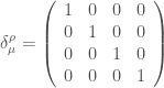
We will use the symbol $g_{\mu\nu}$ for our metric, and we will also often express it as a matrix. For the case of flat spacetime, our metric is given by the Minkowski metric $\eta_{\mu\nu}$ :

$\displaystyle \eta_{\mu\nu}=\left(\begin{array}{cccc}-1&0&0&0\\0&1&0&0\\0&0&1&0\\ 0&0&0&1\end{array}\right)$

We can use the metric to “raise” and “lower” indices. This is done by multiplying the metric and a vector, and summing over a common index (one will be a superscript and the other a subscript). We have introduced the Einstein summation convention in Some Basics of (Quantum) Electrodynamics, where repeated indices always imply summation, unless explicitly stated otherwise, and we will continue to use this convention for posts discussing differential geometry and the theory of relativity.

Here is an example of “lowering” the index of $x^{\nu}$ in flat spacetime using the metric $\eta_{\mu\nu}$ to obtain a new quantity $x_{\mu}$ :

$\displaystyle x_{\mu}=\eta_{\mu\nu}x^{\nu}$

Explicitly, the components of the quantity $x_{\mu}$ are given by $x_{0}=-ct$ , $x_{1}=x$ , $x_{2}=y$ , and $x_{3}=z$ . Note that the “time” component $x_{0}$ has changed sign; this is because $\eta_{00}=-1$ . A quantity such as $x_{\mu}$ , which has a subscript index, is called a covariant vector.

In order to “raise” indices, we need the “inverse metric” $g^{\mu\nu}$ . For the Minkowski metric $\eta_{\mu\nu}$ , the inverse metric $\eta^{\mu\nu}$ has the exact same components as $\eta_{\mu\nu}$ , but for more general metrics this may not be the case. The general procedure for obtaining the inverse metric is to consider the expression

$\eta_{\mu\nu}\eta^{\nu\rho}=\delta_{\mu}^{\rho}$

where $\delta_{\mu}^{\rho}$ is the Kronecker delta, a quantity that can be expressed as the matrix

$\displaystyle \delta_{\mu}^{\rho}=\left(\begin{array}{cccc}1&0&0&0\\0&1&0&0\\0&0&1&0\\ 0&0&0&1\end{array}\right)$ .

As a demonstration of what our notation can do, we recall the formula for the invariant spacetime interval:

$\displaystyle (ds)^2=-(cdt)^2+(dx)^2+(dy)^2+(dz)^2$

Using tensor notation combined with the Einstein summation convention, this can be written simply as

$\displaystyle (ds)^2=\eta_{\mu\nu}dx^{\mu}dx^{\nu}$ .

The Christoffel Symbol and the Covariant Derivative

We now come back to the Christoffel symbol $\Gamma^{\mu}_{\nu\lambda}$ . The idea behind the Christoffel symbol is that it is used to define the covariant derivative $\nabla_{\nu}V^{\mu}$ of a vector $V^{\mu}$ .

The covariant derivative is a very important concept in differential geometry (and not just in Riemannian geometry). When we take derivatives, we are actually comparing two vectors. To further explain what we mean, we recall that individually the components of the vectors can be thought of as functions on the space, and we recall the expression for the derivative from An Intuitive Introduction to Calculus:

$\displaystyle \frac{df}{dx}=\frac{f(x+\epsilon)-f(x)}{(x+\epsilon)-(x)}$ when $\epsilon$ is extremely small (essentially negligible)

More formally, we can write

$\displaystyle \frac{df}{dx}=\lim_{\epsilon\to 0}\frac{f(x+\epsilon)-f(x)}{(x+\epsilon)-(x)}$ .

Therefore, employing the language of partial derivatives, we could have written the following partial derivative of the $\mu$ -th component of an $m$ -dimensional vector $V^{\mu}$ on an $m$ -dimensional space with respect to the coordinate $x^{\nu}$ :

$\displaystyle \frac{\partial V^{\mu}}{\partial x^{\nu}}=\lim_{\Delta x^{\nu}\to 0}\frac{V^{\mu}(x^{1},...,x^{\nu}+\Delta x^{\nu},...,x^{m})-V^{\mu}(x_{1},...,x^{\nu},...,x^{m})}{(x^{\nu}+\Delta x^{\nu})-(x^{\nu})}$

The problem is that we are comparing vectors from different vector spaces. Recall from Vector Fields, Vector Bundles, and Fiber Bundles that we can think of a vector bundle as having a vector space for every point on the base space. The vector $V^{\mu}(x^{1},...,x^{\nu}+\Delta x^{\nu},...,x^{m})$ belongs to the vector space on the point $(x^{1},...,x^{\nu}+\Delta x^{\nu},...,x^{m})$ , while the vector $V^{\mu}(x_{1},...,x^{\nu},...,x^{m})$ belongs to the vector space on the point $(x_{1},...,x^{\nu},...,x^{m})$ . To be able to compare the two vectors we need to “transport” one to the other in the “correct” way, by which we mean parallel transport. Now we have seen in Geometry on Curved Spaces that parallel transport can have weird effects on vectors, and these weird effects are what the Christoffel symbol expresses.

Let $\tilde{V}^{\mu}(x^{1},...,x^{\nu}+\Delta x^{\nu},...,x^{m})$ denote the vector $V^{\mu}(x_{1},...,x^{\nu},...,x^{m})$ parallel transported from its original vector space on $(x_{1},...,x^{\nu},...,x^{m})$ to the vector space on $(x^{1},...,x^{\nu}+\Delta x^{\nu},...,x^{m})$ . The vector $\tilde{V}^{\mu}(x^{1},...,x^{\nu}+\Delta x^{\nu},...,x^{m})$ is given by the following expression:

$\displaystyle \tilde{V}^{\mu}(x^{1},...,x^{\nu}+\Delta x^{\nu},...,x^{m})=V^{\mu}(x_{1},...,x^{\nu},...,x^{m})-V^{\lambda}(x_{1},...,x^{\nu},...,x^{m})\Gamma^{\mu}_{\nu\lambda}(x_{1},...,x^{\nu},...,x^{m})\Delta x^{\nu}$

Therefore the Christoffel symbol provides a “correction” for what happens when we parallel transport a vector from one point to another. This is an example of the concept of a connection, which, like the covariant derivative, is part of more general differential geometry beyond Riemannian geometry. The object that is to be parallel transported may not be a vector, for example when we have more general fiber bundles instead of vector bundles. However, in Riemannian geometry we will usually focus on vector bundles, in particular a special kind of vector bundle called the tangent bundle, which consists of the tangent vectors at a point.

Now there is more than one way to parallel transport a mathematical object, which means that there are many choices of a connection. However, in Riemannian geometry there is a special kind of connection that we will prefer. This is the connection that satisfies the following two properties:

$\displaystyle \Gamma^{\mu}_{\nu\lambda}=\Gamma^{\mu}_{\lambda\nu}$ (torsion-free)

$\displaystyle \nabla_{\rho}g_{\mu\nu}$ (metric compatibility)

The connection that satisfies these two properties is the one that can be obtained from the metric via the following formula:

$\displaystyle \Gamma^{\mu}_{\nu\lambda}=\frac{1}{2}g^{\mu\sigma}(\partial_{\lambda}g_{\mu\sigma}+\partial_{\mu}g_{\sigma\lambda}-\partial_{\sigma}g_{\lambda\mu})$ .

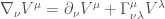
The covariant derivative is then defined as

$\displaystyle \nabla_{\nu}V^{\mu}=\lim_{\Delta x^{\nu}\to 0}\frac{V^{\mu}(x^{1},...,x^{\nu}+\Delta x^{\nu},...,x^{m})-\tilde{V}^{\mu}(x_{1},...,x^{\nu}+\Delta x^{\nu},...,x^{m})}{(x^{\nu}+\Delta x^{\nu})-(x^{\nu})}$ .

We are now comparing vectors belonging to the same vector space, and evaluating the expression above leads to the formula for the covariant derivative:

$\displaystyle \nabla_{\nu}V^{\mu}=\partial_{\nu}V^{\mu}+\Gamma^{\mu}_{\nu\lambda}V^{\lambda}$ .

The Riemann Curvature Tensor

Next we consider the quantity known as the Riemann curvature tensor. It is once again related to parallel transport, in the following manner. Consider parallel transporting a vector $V^{\sigma}$ through an “infinitesimal” distance specified by another vector $A^{\mu}$ , and after that, through another infinitesimal distance specified by a yet another vector $B^{\nu}$ . Then we go parallel transport it again in the opposite direction to $A^{\mu}$ , then finally in the opposite direction to $B^{\nu}$ . The path forms a parallelogram, and when the vector $V^{\sigma}$ returns to its starting point it will then be changed by an amount $\delta V^{\rho}$ . We can think of the Riemann curvature tensor as the quantity that relates all of these:

$\displaystyle \delta V^{\rho}=R^{\rho}_{\ \sigma\mu\nu}V^{\sigma}A^{\mu}B^{\nu}$ .

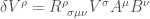
Another way to put this is to consider taking the covariant derivative of the vector $V^{\rho}$ along the same path as described above. The Riemann curvature tensor is then related to this quantity as follows:

$\displaystyle \nabla_{\mu}\nabla_{\nu}V^{\rho}-\nabla_{\nu}\nabla_{\mu}V^{\rho}=R^{\rho}_{\ \sigma\mu\nu}V^{\sigma}$ .

Expanding the left hand side, and using the torsion-free property of the Christoffel symbol, we will find that

$\displaystyle R^{\rho}_{\ \sigma\mu\nu}=\partial_{\mu}\Gamma^{\rho}_{\nu\sigma}-\partial_{\nu}\Gamma^{\rho}_{\mu\sigma}+\Gamma^{\rho}_{\mu\lambda}\Gamma^{\lambda}_{\nu\sigma}-\Gamma^{\rho}_{\nu\lambda}\Gamma^{\lambda}_{\mu\sigma}$ .

For connections other than the torsion-free one that we chose, there will be another part of the expansion of the expression $\nabla_{\mu}\nabla_{\nu}-\nabla_{\nu}\nabla_{\mu}$ called the torsion tensor. For our case, however, we need not worry about it and we can focus on the Riemann curvature tensor.

There is another quantity that can be obtained from the Riemann curvature tensor called the Ricci tensor, denoted by $R_{\mu\nu}$ . It is given by

$\displaystyle R_{\mu\nu}=R^{\lambda}_{\ \mu\lambda\nu}$ .

Following the Einstein summation convention, we sum over the repeated index $\lambda$ , and therefore the resulting quantity will have only two indices instead of four. This is an example of the operation on tensors called contraction. If we raise one index using the metric and contract again, we obtain a quantity called the Ricci scalar, denoted $R$ :

$\displaystyle R=R^{\mu}_{\ \mu}$

Example: The $2$ -Sphere

To provide an explicit example of the concepts discussed, we show their specific expressions for the case of a $2$ -sphere. We will only give the final results here. The explicit computations can be found among the references, but the reader may gain some practice, especially on manipulating tensors, by performing the calculations and checking only the answers here. In any case, since the metric is given, it is only a matter of substituting the relevant quantities into the formulas already given above.

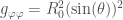
We have already given the expression for the metric of the $2$ -sphere in Geometry on Curved Spaces. We recall that it in matrix form, it is given by (we change our notation for the radius of the $2$ -sphere to $R_{0}$ to avoid confusion with the symbol for the Ricci scalar)

$\displaystyle g_{mn}= \left(\begin{array}{cc}R_{0}^{2}&0\\ 0&R_{0}^{2}\text{sin}(\theta)^{2}\end{array}\right)$

Individually, the components are (we will use $\theta$ and $\varphi$ instead of the numbers $1$ and $2$ for the indices)

$\displaystyle g_{\theta\theta}=R_{0}^{2}$

$\displaystyle g_{\varphi\varphi}=R_{0}^{2}(\text{sin}(\theta))^{2}$

The other components ( $g_{\theta\varphi}$ and $g_{\varphi\theta}$ ) are all equal to zero.

The Christoffel symbols are therefore given by

$\displaystyle \Gamma^{\theta}_{\varphi\varphi}=-\text{sin}(\theta)\text{cos}(\theta)$

$\displaystyle \Gamma^{\varphi}_{\theta\varphi}=\text{cot}(\theta)$

$\displaystyle \Gamma^{\varphi}_{\varphi\theta}=\text{cot}(\theta)$

The other components ( $\Gamma^{\theta}_{\theta\theta}$ , $\Gamma^{\theta}_{\theta\varphi}$ , $\Gamma^{\theta}_{\varphi\theta}$ , $\Gamma^{\varphi}_{\theta\theta}$ , and $\Gamma^{\varphi}_{\varphi\varphi}$ ) are all equal to zero.

The components of the Riemann curvature tensor are given by

$\displaystyle R^{\theta}_{\ \varphi\theta\varphi}=(\text{sin}(\theta))^{2}$

$\displaystyle R^{\theta}_{\ \varphi\varphi\theta}=-(\text{sin}(\theta))^{2}$

$\displaystyle R^{\varphi}_{\ \theta\theta\varphi}=-1$

$\displaystyle R^{\varphi}_{\ \theta\varphi\theta}=1$

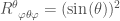
The other components (there are still twelve of them, so I won’t bother writing all their symbols down here anymore) are all equal to zero.

The components of the Ricci tensor is

$\displaystyle R_{\theta\theta}=1$

$\displaystyle R_{\varphi\varphi}=(\text{sin}(\theta))^{2}$

The other components ( $R_{\theta\varphi}$ and $R_{\varphi\theta}$ ) are all equal to zero.

Finally, the Ricci scalar is

$\displaystyle R=\frac{2}{R_{0}^{2}}$

We note that the larger the radius of the $2$ -sphere, the smaller the curvature. We can see this intuitively, for example, when it comes to the surface of our planet, which appears flat because the radius is so large. If our planet was much smaller, this would not be the case.

Bonus: The Einstein Field Equations of General Relativity

Given what we have discussed in this post, we can now write down here the expression for the Einstein field equations (also known simply as Einstein’s equations) of general relativity. It is given in terms of the Ricci tensor and the metric (of spacetime) via the following equation:

$\displaystyle R_{\mu\nu}-\frac{1}{2}Rg_{\mu\nu}+\Lambda g_{\mu\nu}=\frac{8\pi}{c^{4}} GT_{\mu\nu}$

where $G$ is the gravitational constant, the same constant that appears in Newton’s law of universal gravitation (which is approximated by Einstein’s equations at certain limiting conditions), $c$ is the speed of light in a vacuum, and $T_{\mu\nu}$ is the energy-momentum tensor (also known as the stress-energy tensor), which gives the “density” of energy and momentum, as well as certain other related concepts, such as the pressure and shear stress. The symbol $\Lambda$ refers to what is known as the cosmological constant, which was not there in Einstein’s original formulation but later added to support his view of an unchanging universe. Later, with the dawn of George Lemaitre’s theory of an expanding universe, later known as the Big Bang theory, the cosmological constant was abandoned. More recently, the universe was found to not only be expanding, but expanding at an accelerating rate, necessitating the return of the cosmological constant, with an interpretation in terms of the “vacuum energy”, also known as “dark energy”. Today the nature of the cosmological constant remains one of the great mysteries of modern physics.

Bonus: Connection and Curvature in Quantum Electrodynamics

The concepts of connection and curvature also appear in quantum field theory, in particular quantum electrodynamics (see Some Basics of (Quantum) Electrodynamics). It is the underlying concept in gauge theory, of which quantum electrodynamics is probably the simplest example. However, it is an example of differential geometry which does not make use of the metric. We consider a fiber bundle, where the base space is flat spacetime (also known as Minkowski spacetime), and the fiber is $\text{U}(1)$ , which is the group formed by the complex numbers with magnitude equal to $1$ , with law of composition given by multiplication (we can also think of this as a circle).

We want the group $\text{U}(1)$ to act on the wave function (or field operator) $\psi(x)$ , so that the wave function has a “phase”, i.e. we have $e^{i\phi(x)}\psi(x)$ , where $e^{i\phi(x)}$ is a complex number which depends on the location $x$ in spacetime. Note that therefore different values of the wave function at different points in spacetime will have different values of the “phase”. In order to compare, them, we need a connection and a covariant derivative.

The connection we want is given by

$\displaystyle i\frac{q}{\hbar c}A_{\mu}$

where $q$ is the charge of the electron, $\hbar$ is the normalized Planck’s constant, $c$ is the speed of light in a vacuum, and $A_{\mu}$ is the four-potential of electrodynamics.

The covariant derivative (here written using the symbol $D_{\mu}$ )is

$\displaystyle D_{\mu}\psi(x)=\partial_{\mu}\psi(x)+i\frac{q}{\hbar c}A_{\mu}\psi(x)$

We will also have a concept analogous to the Riemann curvature tensor, called the field strength tensor, denoted $F_{\mu\nu}$ . Of course, our “curvature” in this case is not the literal curvature of spacetime, as we have already specified that our spacetime is flat, but an abstract notion of “curvature” that specifies how the phase of our wavefunction changes as we move around the spacetime. This field strength tensor is given by the following expression:

$F_{\mu\nu}=\partial_{\mu}A_{\nu}-\partial_{\nu}A_{\mu}$

This may be compared to the expression for the Riemann curvature tensor, where the connection is given by the Christoffel symbols. The first two terms of both expressions are very similar. The difference is that the expression for the Riemann curvature tensor has some extra terms that the expression for the field strength tensor does not have. However, a generalization of this procedure for quantum electrodynamics to groups other than $\text{U}(1)$ , called Yang-Mills theory, does feature extra terms in the expression for the field strength tensor that perhaps makes the two more similar.

The concepts we have discussed here can be used to derive the theory of quantum electrodynamics simply from requiring that the Lagrangian (from which we can obtain the equations of motion, see also Lagrangians and Hamiltonians) be invariant under $\text{U}(1)$ transformations, i.e. even if we change the “phase” of the wave function at every point the Lagrangian remains the same. This is an example of what is known as gauge symmetry. Generalized to other groups such as $\text{SU}(2)$ and $\text{SU}(3)$ , this is the idea behind gauge theories, which include Yang-Mills theory and leads to the standard model of particle physics.