Hecke Operators

November 30, 2020December 1, 2020 / Anton Hilado / 7 Comments

A Hecke operator is a certain kind of linear transformation on the space of modular forms or cusp forms (see also Modular Forms) of a certain fixed weight $k$ . They were originally used (and now named after) Erich Hecke, who used them to study L-functions (see also Zeta Functions and L-Functions) and in particular to determine the conditions for whether an L-series $\sum_{n=1}^{\infty}a_{n}n^{-s}$ has an Euler product. Together with the meromorphic continuation and the functional equation, these are the important properties of the Riemann zeta function, which L-functions are supposed to be generalizations of. Hecke’s study was inspired by the work of Bernhard Riemann on the zeta function.

An example of a Hecke operator is the one commonly denoted $T_{p}$ , for $p$ a prime number. To understand it conceptually, we must take the view of modular forms as functions on lattices. This is equivalent to the definition of modular forms as functions on the upper half-plane, if we recall that a lattice $\Lambda$ can also be expressed as $\mathbb{Z}+\tau\mathbb{Z}$ where $\tau$ is a complex number in the upper half-plane (see also The Moduli Space of Elliptic Curves).

In this view a modular form is a function on the space of lattices on $\mathbb{C}$ such that

$f(\mathbb{Z}+\tau\mathbb{Z})$ is holomorphic as a function on the upper half-plane
$f(\mathbb{Z}+\tau\mathbb{Z})$ is bounded as $\tau$ goes to $i\infty$
$f(\mu\Lambda)=\mu^{-k}f(\Lambda)$ for some nonzero complex number $\mu$ , and $k$ is the weight of the modular form

Now we define the Hecke operator $T_{p}$ by what it does to a modular form $f(\Lambda)$ of weight $k$ as follows:

$\displaystyle T_{p}f(\Lambda)=p^{k-1}\sum_{\Lambda'\subset \Lambda}f(\Lambda')$

where $\Lambda'$ runs over the sublattices of $\Lambda$ of index $p$ . In other words, applying $T_{p}$ to a modular form gives back a modular form whose value on a lattice $\Lambda$ is the sum of the values of the original modular form on the sublattices of $\Lambda$ of index $p$ , times some factor that depends on the Hecke operator and the weight of the modular form.

Hecke operators are also often defined via their effect on the Fourier expansion of a modular form. Let $f(\tau)$ be a modular form of weight $k$ whose Fourier expansion is given by $\sum_{n=0}^{\infty}a_{i}q^{i}$ , where we have adopted the convention $q=e^{2\pi i \tau}$ which is common in the theory of modular forms (hence this Fourier expansion is also known as a $q$ -expansion). Then the effect of a Hecke operator $T_{p}$ is as follows:

$\displaystyle T_{p}f(\tau)=\sum_{n=0}^{\infty}(a_{pn}+p^{k-1}a_{n/p})q^{n}$

where $a_{n/p}=0$ when $p$ does not divide $n$ . To see why this follows from our first definition of the Hecke operator, we note that if our lattice is given by $\mathbb{Z}+\tau\mathbb{Z}$ , there are $p+1$ sublattices of index $p$ : There are $p$ of these sublattices given by $p\mathbb{Z}+(j+\tau)\mathbb{Z}$ for $j$ ranging from $0$ to $p-1$ , and another one given by $\mathbb{Z}+(p\tau)\mathbb{Z}$ . Let us split up the Hecke operators as follows:

$\displaystyle T_{p}f(\mathbb{Z}+\tau\mathbb{Z})=p^{k-1}\sum_{j=0}^{p-1}f(p\mathbb{Z}+(j+\tau)\mathbb{Z})+p^{k-1}f(\mathbb{Z}+p\tau\mathbb{Z})=\Sigma_{1}+\Sigma_{2}$

where $\Sigma_{1}=p^{k-1}\sum_{j=0}^{p-1}f(p\mathbb{Z}+(j+\tau)\mathbb{Z})$ and $\Sigma_{2}=p^{k-1}f(\mathbb{Z}+p\tau\mathbb{Z})$ . Let us focus on the former first. We have

$\displaystyle \Sigma_{1}=p^{k-1}\sum_{j=0}^{p-1}f(p\mathbb{Z}+(j+\tau)\mathbb{Z})$

But applying the third property of modular forms above, namely that $f(\mu\Lambda)=\mu^{-k}f(\Lambda)$ with $\mu=p$ , we have

$\displaystyle \Sigma_{1}=p^{-1}\sum_{j=0}^{p-1}f(\mathbb{Z}+((j+\tau)/p)\mathbb{Z})$

Now our argument inside the modular forms being summed are in the usual way we write them, except that instead of $\tau$ we have $((j+\tau)/p)$ , so we expand them as a Fourier series

$\displaystyle \Sigma_{1}=p^{-1}\sum_{j=0}^{p-1}\sum_{n=0}^{\infty}a_{n}e^{2\pi i n((j+\tau)/p)}$

We can switch the summations since one of them is finite

$\displaystyle \Sigma_{1}=p^{-1}\sum_{n=0}^{\infty}\sum_{j=0}^{p-1}a_{n}e^{2\pi i n((j+\tau)/p)}$

The inner sum over $j$ is zero unless $p$ divides $n$ , in which case the sum is equal to $p$ . This gives us

$\displaystyle \Sigma_{1}=p^{-1}\sum_{n=0}^{\infty}a_{pn}q^{n}$

where again $q=e^{2\pi i \tau}$ . Now consider $\Sigma_{2}$ . We have

$\displaystyle \Sigma_{2}=p^{k-1}f(\mathbb{Z}+p\tau\mathbb{Z})$

Expanding the right hand side into a Fourier series, we have

$\displaystyle \Sigma_{2}=p^{k-1}\sum_{n}a_{n}e^{2\pi i n p\tau}$

Reindexing, we have

$\displaystyle \Sigma_{2}=p^{k-1}\sum_{n}a_{n/p}q^{n}$

and adding together $\Sigma_{1}$ and $\Sigma_{2}$ gives us our result.

The Hecke operators can be defined not only for prime numbers, but for all natural numbers, and any two Hecke operators $T_{m}$ and $T_{n}$ commute with each other. They preserve the weight of a modular form, and take cusp forms to cusp forms (this can be seen via their effect on the Fourier series). We can also define Hecke operators for modular forms with level structure, but it is more complicated and has some subtleties when for the Hecke operator $T_{n}$ we have $n$ sharing a common factor with the level.

If a cusp form $f$ is an eigenvector for a Hecke operator $T_{n}$ , and it is normalized, i.e. its Fourier coefficient $a_{1}$ is equal to $1$ , then the corresponding eigenvalue of the Hecke operator $T_{n}$ on $f$ is precisely the Fourier coefficient $a_{n}$ .

Now the Hecke operators satisfy the following multiplicativity properties:

$T_{m}T_{n}=T_{mn}$ for $m$ and $n$ mutually prime
$T_{p^{n}}T_{p}=T_{p^{n+1}}+p^{k-1}T_{p}$ for $p$ prime

Suppose we have an L-series $\sum_{n}a_{n}n^{-s}$ . This L-series will have an Euler product if and only if the coefficients $a_{n}$ satisfy the following:

$a_{m}a_{n}=a_{mn}$ for $m$ and $n$ mutually prime
$a_{p^{n}}T_{p}=a_{p^{n+1}}+p^{k-1}a_{p}$ for $p$ prime

Given that the Fourier coefficients of a normalized Hecke eigenform (a normalized cusp form that is a simultaneous eigenvector for all the Hecke operators) are the eigenvalues of the Hecke operators, we see that the L-series of a normalized Hecke eigenform has an Euler product.

In addition to the Hecke operators $T_{n}$ , there are also other closely related operators such as the diamond operator $\langle n\rangle$ and another operator denoted $U_{p}$ . These and more on Hecke operators, such as other ways to define them with double coset operators or Hecke correspondences will hopefully be discussed in future posts.

References:

Hecke Operator on Wikipedia

Modular Forms by Andrew Snowden

Congruences between Modular Forms by Frank Calegari

A First Course in Modular Forms by Fred Diamond and Jerry Shurman

Advanced Topics in the Arithmetic of Elliptic Curves by Joseph H. Silverman

Iwasawa theory, p-adic L-functions, and p-adic modular forms

November 30, 2020December 7, 2022 / Anton Hilado / 2 Comments

In Bernoulli Numbers, Fermat’s Last Theorem, and the Riemann Zeta Function, we introduced the Kubota-Leopold $p$ -adic L-function, which encodes the congruences discovered by Kummer between special values of the Riemann zeta function. In this post, we will connect them to Iwasawa theory and $p$ -adic modular forms.

Let us start with a little introduction to Iwasawa theory. Consider the Galois group $\text{Gal}(\mathbb{Q}(\mu_{p^{\infty}})/\mathbb{Q})$ , where $\mathbb{Q}(\mu_{p^{\infty}})$ is the extension of the rational numbers $\mathbb{Q}$ obtained by adjoining all the $p$ -th-power roots of unity to $\mathbb{Q}$ . This Galois group is isomorphic to $\mathbb{Z}_{p}^{\times}$ , the group of units of the $p$ -adic integers $\mathbb{Z}_p$ .

The group $\mathbb{Z}_{p}^{\times}$ decomposes into the product of a group isomorphic to $1+p\mathbb{Z}_{p}$ and a group isomorphic to $(p-1)$ -th roots of unity. Let $\Gamma$ be the subgroup of this Galois group isomorphic to $1+p\mathbb{Z}_{p}$ . The Iwasawa algebra is defined to be the group ring $\mathbb{Z}_{p}[[\Gamma]]$ , which also happens to be isomorphic to the power series ring $\mathbb{Z}_{p}[[T]]$ .

The interest in the Iwasawa algebra comes from the fact that many important objects of interest in number theory are modules over the Iwasawa algebra, and such modules have a structure that makes them easy to study. For instance, the inverse limit of the p-part of the ideal class groups of cyclotomic fields is such a module. The “main conjecture of Iwasawa theory“, a high-powered version of Kummer’s theorem that relates ideal class groups and Bernoulli numbers, describes this module. Namely, the main conjecture of Iwasawa theory states that as a module over the Iwasawa algebra, the inverse limit of the p-part of the ideal class groups of cyclotomic fields has a characteristic ideal generated by none other than the Kubota-Leopoldt $p$ -adic L-function!

Let us describe more the relation between the Iwasawa algebra and the Kubota-Leopoldt zeta function by relating them to measures. Our measure here takes functions on the group $\mathbb{Z}_p^{\times}$ and gives an element of $\mathbb{Z}_{p}$ . This should remind us of measures and integrals in real analysis, except instead of our functions being on $\mathbb{R}$ , they are on the group $\mathbb{Z}_{p}^{\times}$ , and instead of taking values in $\mathbb{R}$ , they take values in $\mathbb{Z}_{p}$ . This is just an example of a more general kind of measure.

Now these measures are actually in one-to-one correspondence with the elements of the Iwasawa algebra!

The Iwasawa algebra is $\mathbb{Z}_{p}[[\Gamma]]$ , and note that $\Gamma$ is a subset of $\mathbb{Z}_{p}^{\times}$ . Suppose we have an element of the Iwasawa algebra. We define the corresponding measure by saying what it does to a function $f$ on $\mathbb{Z}_{p}^{\times}$ . Note that if we extend this function linearly, we can evaluate it on the element of the Iwasawa algebra and get an element of $\mathbb{Z}_{p}^{\times}$ . Thus we define our measure by evaluation. The other direction is a bit more involved, but given the measure, we build an element of the Iwasawa algebra by exploiting the profinite nature of $\mathbb{Z}_{p}^{\times}$ , which means the measure was built from functions on the finite pieces of it.

Now we know how the Iwasawa algebra and measures are related, what about the Kubota-Leopoldt zeta function? For those we must now take a detour through $p$ -adic modular forms, in particular $p$ -adic Eisenstein series.

The reason modular forms are brought into this is that the value of the zeta function at $1-k$ shows up in the constant term in the Fourier expansion of the Eisenstein series $G_{k}$ :

$\displaystyle G_{k}(\tau):=\frac{\zeta(1-k)}{2}+\sum_{n=1}^{\infty}\left(\sum_{d\vert n}d^{k-1}\right)q^{n}$

where $q=e^{2\pi i \tau}$ , as is common convention in the theory (hence the Fourier expansion is also known as the $q$ -expansion). This Eisenstein series $G_{k}$ is a modular form of weight $k$ . A similar relationship holds between the Kubota-Leopoldt $p$ -adic L-function and $p$ -adic Eisenstein series, the latter of which is an example of a $p$ -adic modular form. We will define this now. Let $f$ be a modular form defined over $\mathbb{Q}$ . This means that, when we consider its Fourier expansion

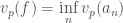
$\displaystyle f(\tau)=\sum_{n=0}^{\infty}a_{n}q^{n}$ ,

the coefficients $a_{n}$ are rational numbers. We define a $p$ -adic valuation on the space of modular form by taking the biggest power of $p$ among the coefficients $a_{n}$ , i.e.

$\displaystyle v_{p}(f)=\inf_{n} v_{p}(a_{n})$

We recall that the bigger the power of $p$ dividing a rational number, the smaller its $p$ -adic valuation. This lets us consider the limit of a sequence. A $p$ -adic modular form is the limit of a sequence of classical modular forms.

The weight of a $p$ -adic modular form is the limit of the weights of the classical ones of which it is the limit. Serre showed that for classical modular forms $f$ and $g$ , if the $p$ -adic valuation

$\displaystyle v(f-g)>=v(f)+m$

for some $m$ , then the weights of $f$ and $g$ will be congruent mod $(p-1)p^m$ .

This implies that the weight of a $p$ -adic modular form takes values in the inverse limit of $\mathbb{Z}/(p-1)p^{m}\mathbb{Z}$ , which is isomorphic to the product of $\mathbb{Z}_{p}$ and $(p-1)\mathbb{Z}$ . Here is where measures come in – this space of weights can be identified with characters of $\mathbb{Z}_{p}^{\times}$ , i.e. a weight $k$ is a function on $\mathbb{Z}_{p}^{\times}$ and being such a function, it is an input for a measure!

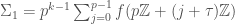
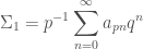
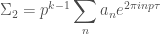
Now, we will create a measure, with a bit of a twist. Given a weight $k$ , we can build a $p$ -adic Eisenstein series of weight $k$ (recall that this is a limit of classical Eisenstein series):

$\displaystyle G_{k}^{*}:=\varinjlim_{i}G_{k_{i}}$

We think of this as a “measure” that takes a weight $k$ (again recall that the weight $k$ is a character, i.e. a function on $\mathbb{Z}_{p}$ ) and gives a weight $k$ Eisenstein series, i.e an “Eisenstein measure“. But the value of the Kubota-Leopoldt zeta function at $1-k$ is the constant in the Fourier expansion! Therefore, if we take the constant term of this p-adic Eisenstein series, we have a good old measure, a recipe for taking a function on $\mathbb{Z}_{p}$ (the weight $k$ ) and giving us an element of $\mathbb{Z}_{p}$ . But by our earlier discussion, this is an element of the Iwasawa algebra!

There are some subtleties I swept under the rug, but to summarize – important objects in number theory are modules over the Iwasawa algebra. $p$ -adic L-functions which interpolate L-functions at special values are elements of the Iwasawa algebra.

This is a modern, high-powered version of Kummer’s discovery that relates certain ideal class groups and Bernoulli numbers (which are special values of the Riemann zeta function). The Eisenstein measure, which gives a p-adic modular form when evaluated at a certain weight, leads to the notion of a “Hida family“, a “p-adic family” of p-adic modular forms. But that discussion is for another time!

References:

Iwasawa theory on Wikipedia

Iwasawa algebra on Wikipedia

p-adic L-function on Wikipedia

Main conjecture of Iwasawa theory on Wikipedia

An introduction to Eisenstein measures by E. E. Eischen

Modular curves and cyclotomic fields by Romyar Sharifi

Desde Fermat, Lamé y Kummer hasta Iwasawa: Una introducción a la teoría de Iwasawa (in Spanish) by Álvaro Lozano-Robledo

Bernoulli Numbers, Fermat’s Last Theorem, and the Riemann Zeta Function

November 28, 2020 / Anton Hilado / 1 Comment

The Bernoulli numbers are the Taylor series coefficients of the function

$\displaystyle \frac{x}{e^{x}-1}$ .

The $n$ -th Bernoulli number $B_{n}$ is zero for odd $n$ , except for $n=1$ , where it is equal to $-1/2$ . For the first few even numbers, we have

$\displaystyle B_0=1,\; B_{2}=\frac{1}{6}, \; B_{4}=-\frac{1}{30}, \; B_6=\frac{1}{42}, \; B_{8}=-\frac{1}{30}, \; B_{10}=\frac{5}{66}$ .

Bernoulli numbers have many interesting properties, and many mathematicians have studied them for a very long time. They are named after Jacob Bernoulli, but were also studied by Seki Takakazu in Japan at around the same time (end of 17th/beginning of 18th century). In this post I want to focus more on the work of Ernst Edouard Kummer, more than a century after Bernoulli and Takakazu.

We’re going to come back to Bernoulli numbers later, but for now let’s talk about something completely different – Fermat’s Last Theorem, which Kummer was working on. In the time of Kummer, a proposal to study Fermat’s Last Theorem by factoring both sides of the famous equation into linear terms. Just as $x^2+y^2$ factors into

$\displaystyle x^2+y^2=(x+iy)(x-iy)$ ,

we would have that $x^{p}+y^{p}$ also factors into

$\displaystyle x^{p}+y^{p}=(x+\zeta_{p}y)(x+\zeta_{p}^{2} y)...(x+\zeta_{p}^{p-1} y)$

where $\zeta_{p}$ is a $p$ -th root of unity.

However, there is a problem. In these kinds of numbers where $p$ -th roots of unity are adjoined, factorization may not be unique! Hence Kummer developed the theory of “ideals” to study this (see also The Fundamental Theorem of Arithmetic and Unique Factorization).

Unique factorization does not work with the numbers themselves, but it works with ideals (this is true for number fields, since they form what is called a “Dedekind domain”). Hence the original name of ideals was “ideal numbers”. To number fields we associate an “ideal class group“. If this group has only one element, unique factorization holds. If not, then things can get complicated. The ideal class group (together with the Galois group) is probably the most important group in number theory.

Kummer found that if $p$ is a “regular prime“, i.e. if p does not divide the number of elements of the ideal class group (also known as the class number) of the “ $p$ -th cyclotomic field” (the rational numbers with $p$ -th roots of unity adjoined), then Fermat’s Last Theorem is true for $p$ .

Let’s go back to Bernoulli numbers now – Kummer also found that a prime $p$ is regular if and only if it does not divide the numerator for the nth Bernoulli number, for all $n$ less than $p-1$ . In other words, Kummer proved Fermat’s Last Theorem for prime exponents not dividing the numerators of Bernoulli numbers! Fermat’s Last Theorem has now been proved in all cases, but the work of Kummer remains influential.

So we’ve related Bernoulli numbers to ideal class groups and the very famous Fermat’s Last Theorem. Now let us relate Bernoulli numbers to another very famous thing in math – the Riemann zeta function (see also Zeta Functions and L-Functions).

It is known that the Bernoulli numbers are related to values of the Riemann zeta function at the negative integers (so we need the analytic continuation to do this) by the following equation: $B_n=n \zeta(1-n)$ for $n$ greater than or equal to $1$ .

Now, Kummer also discovered that Bernoulli numbers satisfy certain congruences modulo powers of a prime $p$ , in particular

$\displaystyle \frac{B_{m}}{m}\equiv \frac{B_{n}}{n} \mod p$

where $m$ and $n$ are positive even integers neither of which are divisible by $(p-1)$ , and $m\equiv n \mod (p-1)$ . Here congruence for two rational numbers $\frac{a}{b}$ and $\frac{c}{d}$ means that $ad$ is congruent to $cd$ mod $p$ .

We also have a more general congruence for bigger powers of $p$ :

$\displaystyle (1-p^{m-1})\frac{B_{m}}{m}\equiv (1-p^{n-1})\frac{B_{n}}{n} \mod p^{a+1}$

where $m$ and $n$ are positive even integers neither of which are divisible by $(p-1)$ , and $m\equiv n \mod \varphi(p^{a}+1)$ , $\varphi^{a}+1$ being the number of positive integers less than $p^{a+1}$ that are also mutually prime to it.

By by our earlier discussion, this means the special values of the Riemann zeta function also satisfy congruences modulo powers of $p$ .

Congruences modulo powers of $p$ is encoded in modern language by the “ $p$ -adic numbers” (see also Valuations and Completions) introduced by Kurt Hensel near the end of the 19th century. The congruences between the special values of the Riemann zeta function is now similarly encoded in a $p$ -adic analytic function known as the Kubota-Leopoldt $p$ -adic L-function.

So again, to summarize the story so far – Bernoulli numbers are related to the ideal class group and also to the special values of the Riemann zeta function, and bridge the two subjects.

If this reminds you of the analytic class number formula, well in fact that is one of the ingredients in the proof of Kummer’s result relating regular primes and the Bernoulli numbers. Moreover, the information that they encode is related to divisibility or congruence modulo primes or their powers. This is where the $p$ -adic L-functions come in.

The Bernoulli numbers also appear in the constant term of the Fourier expansion of Eisenstein series. The Eisenstein series is an example of a modular form (see also Modular Forms), which gives us Galois representations. The Galois group, on the other hand is related to the ideal class group by class field theory (see also Some Basics of Class Field Theory). So this is one way to create the bridge between the two concepts. In fact, this was used to prove the Herbrand-Ribet theorem, a stronger version of Kummer’s result.

So we also have modular forms in the picture. In modern research all of these are deeply intertwined – ideal class groups, zeta functions, congruences, and modular forms.

References:

Bernoulli number on Wikipedia

Riemann zeta function on Wikipedia

Kummer’s congruence on Wikipedia

p-adic L-function on Wikipedia

Herbrand-Ribet theorem on Wikipedia

Bernoulli numbers, Hurwitz numbers, p-adic L-functions and
Kummer’s criterion by Alvaro Lozano-Robledo

An introduction to Eisenstein measures by E. E. Eischen

How can we construct abelian Galois extensions of basic number
fields? by Barry Mazur