Zeta Functions and L-Functions

This is my first post on this blog with actual content, and it’s an attempt to strike a balance between the two kinds of posts I want to make on this blog: expository articles, and personal notes on concepts I’m still trying to understand. It’s also going to feature a bit more of history as compared to actual technical stuff. As this blog continues to grow, I hope to write more of the latter. As of the moment, however, I hope understanding will be given for the lack of rigor on this blog. I will try to post lots of references to make up for it.

The Riemann zeta function is probably known to many people. After all, there is a million dollar prize attached to a problem involving it, known as the Riemann hypothesis, which I will not discuss yet in this post. Instead, first I will note that despite the name, it was not Bernhard Riemann who first discovered the Riemann zeta function. It was already known to Leonhard Euler, who used it to study the prime numbers. Bernhard Riemann’s later work with the Riemann zeta function was for a similar purpose to Euler’s – Riemann used it to give a formula for the number of primes less than a given number. Now that we have given a bit of history of the Riemann zeta function and what it is useful for, we now present its most basic form:

$\displaystyle \zeta(s)=\sum_{n=0}^{\infty} \frac{1}{n^{s}}=\frac{1}{1^{s}}+\frac{1}{2^{s}}+\frac{1}{3^{s}}+...$

The connection with prime numbers comes from the fact that aside from being expressed as an infinite sum, it can also be expressed as an infinite product, called the Euler product:

$\displaystyle \zeta(s)=\prod_{p} \frac{1}{1-p^{-s}}=\bigg(\frac{1}{1-2^{-s}}\bigg)\bigg(\frac{1}{1-3^{-s}})\bigg(\frac{1}{1-5^{-s}}\bigg)...$

where p runs over all prime numbers.

For $s=2$ for example, we have

$\displaystyle \zeta(2)=\sum_{n=0}^{\infty} \frac{1}{n^{2}}=\frac{1}{1^{2}}+\frac{1}{2^{2}}+\frac{1}{3^{2}}+...=1+\frac{1}{4}+\frac{1}{9}+...$

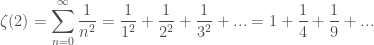
This series converges to the value

$\displaystyle \zeta(2)=\frac{\pi^{2}}{6}$ .

One can see that for some values of $s$ , the infinite series does not converge. However, from complex analysis we have the concept of analytic continuation, which gives a “substitute” for the Riemann zeta function which is equal to the “original” Riemann zeta function wherever it was defined, and yet “continues” it to where it was not defined before. When we have performed this analytic continuation, the “new” Riemann zeta function (which, by the way, is usually written as a complicated expression involving integrals and gamma functions) will then be defined for all values of $s$ except for $s=1$ .

So while the “original” (infinite series) Riemann zeta function diverges for $s=0$ and $s=-1$ , with the “new” (integrals and gamma functions) Riemann zeta function obtained from analytic continuation we have

$\displaystyle \zeta(0)=-\frac{1}{2}$

$\displaystyle \zeta(-1)=-\frac{1}{12}$

If we insist on writing the Riemann zeta function in the “original” infinite series form, this leads to the following very weird results:

$\displaystyle \zeta(0)=\frac{1}{1^{0}}+\frac{1}{2^{0}}+\frac{1}{3^{0}}+...=1+1+1+...=-\frac{1}{2}$

$\displaystyle \zeta(-1)=\frac{1}{1^{-1}}+\frac{1}{2^{-1}}+\frac{1}{3^{-1}}+...=1+2+3+...=-\frac{1}{12}$

Perhaps in some future post I will expound more on these weird results and the method of analytic continuation from which they originate.

While Riemann was doing his work, another great mathematician, Peter Gustav Lejeune Dirichlet, was generalizing the Riemann zeta function to solve another problem involving primes. Namely, what Dirichlet proved was that in an arithmetic progression of positive integers where the first term and the increment are mutually prime, an infinite number of the terms of the progression are prime numbers. For example, consider the infinite arithmetic progression

$\displaystyle 5, 8, 11, 14, 17, 20, 23, 26, 29, 32,...$

The prime numbers here are

$\displaystyle 5, 11, 17, 23, 29,...$ .

What Dirichlet proved is that there are an infinite number of these prime numbers in the infinite arithmetic progression, even though I wrote down only five. Besides, it is quite difficult to identify whether a number is prime or composite when the number is very large. But Dirichlet was able to prove, for sure, that there is an infinite number of them in the progression. And in order to perform this feat Dirichlet had to “generalize” the Riemann zeta function.

But what do we mean by Dirichlet “generalizing” the Riemann zeta function? First we make an analogy between geometric series and power series.

An (infinite) geometric series is a series of the form

$\displaystyle \sum_{n=0}^{\infty}x^{n}$

while a power series is a series of the form

$\displaystyle \sum_{n=0}^{\infty}a_{n}x^{n}$

where the coefficients $a_{n}$ are to be determined by what kind of power series we have. For a Taylor series of a function $f(x)$ at $x=0$ , for example,

$\displaystyle a_{n}=\frac{f^{(n)}(0)}{n!}$

where $f^{(n)}(0)$ is the n-th derivative of $f(x)$ at $x=0$ .

Now we can see that a geometric series is just a power series where $a_{n}=1$ for all $n$ .

Now we go back to Dirichlet’s generalization of the Riemann zeta function, which we now refer to as “L-functions”. An L-function starts out as a Dirichlet series, an infinite series of the form

$\displaystyle \sum_{n=0}^{\infty} \frac{a_{n}}{n^{s}}$ .

So the Riemann zeta function is just a Dirichlet series where $a_{n}=1$ for all $n$ .

Just like in the case of power series, the coefficients $a_{n}$ are determined by special methods. For the problem Dirichlet was considering, what he needed was what we now refer to as a Dirichlet character, which we write using the symbol $\chi(n)$ . The Dirichlet character has some special properties – for example, the Dirichlet character is periodic, i.e. $\chi(n+k)=\chi(n)$ for some number $k$ which we call the period and $\chi(n)=0$ whenever $n$ and the $k$ are not mutually prime, i.e. they have a common factor aside from $1$ . Also, the Dirichlet character is multiplicative, which means that $\chi(mn)=\chi(m)\chi(n)$ .

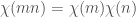
So now we express the above series, which we now refer to as an “L-series”, as

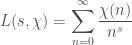
$\displaystyle L(s,\chi)=\sum_{n=0}^{\infty} \frac{\chi(n)}{n^{s}}$ .

L-series, like the Riemann zeta function, can also be expressed as an Euler product. The analytic continuation of the L-series is then what we call an L-function.

I guess that’s it for now, even though we hardly accomplished anything except revisit a little history and get a little sample of the properties of the Riemann zeta function and the Dirichlet L-functions. In the future I guess I’ll make more posts regarding zeta functions and L-functions (I’ll mention at this point that there is another important generalization of the Riemann zeta function, the Dedekind zeta function) including perhaps how they were used to perform the accomplishments that brought fame to the mathematicians these functions are now named after.

Finally, some references:

Riemann Zeta Function on Wikipedia

Dirichlet L-Function on Wikipedia

Riemann’s Zeta Function by Harold M. Edwards

A Classical Introduction to Modern Number Theory by Kenneth Ireland and Michael Rosen

3 thoughts on “Zeta Functions and L-Functions”

Pingback: The Riemann Hypothesis for Curves over Finite Fields | Theories and Theorems
Pingback: Bernoulli Numbers, Fermat’s Last Theorem, and the Riemann Zeta Function | Theories and Theorems
Pingback: Hecke Operators | Theories and Theorems

Theories and Theorems

Math and Physics for Everyone

Zeta Functions and L-Functions

3 thoughts on “Zeta Functions and L-Functions”

Leave a Reply Cancel reply

Share this:

Like this:

3 thoughts on “Zeta Functions and L-Functions”

Leave a Reply Cancel reply