The Riemann Hypothesis for Curves over Finite Fields

The Riemann hypothesis is one of the most famous open problems in mathematics. Not only is there a million dollar prize currently being offered by the Clay Mathematical Institute for its solution, it also has a very long and interesting history spanning over a century and a half. It is part of many famous “lists” of open problems such as the famous 23 problems of David Hilbert, the 18 problems of Stephen Smale, and the 7 “millennium” problems of the aforementioned Clay Mathematical Institute.

The attention and reverence given to the Riemann hypothesis by the mathematical community is not without good reason. The problem originated in the paper “On the Number of Primes Less Than a Given Magnitude” by the mathematician Bernhard Riemann, where he applied the recently developed theory of complex analysis to number theory, in particular to come up with a function \pi(x) that counts the number of prime numbers less than x. The zeroes of the Riemann zeta function figure into the formula for this “prime counting function” \pi(x), and the Riemann hypothesis is a conjecture that concerns these zeroes. Aside from the knowledge about the prime numbers that a solution of the Riemann hypothesis will give us, it is hoped for that efforts toward this solution will lead to developments in mathematics that may be of interest to us for reasons much bigger, and perhaps outside of, the original motivations.

In the 1940’s, the mathematician Andre Weil solved a version of the Riemann hypothesis, which applies to the Riemann zeta function over finite fields. The ideas that Weil developed for solving this version of the Riemann hypothesis has led to many important developments in modern mathematics, whose applications are not limited to the original problem only. It is these ideas that we discuss in this post. But before we can give the statement of the Riemann hypothesis over finite fields (which is almost identical to that of the original Riemann hypothesis), we first review some concepts regarding zeta functions.

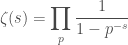
We have discussed zeta functions before in  Zeta Functions and L-Functions. We recall that the Riemann zeta function is given by the formula

\displaystyle \zeta(s)=\sum_{n=1}^{\infty}\frac{1}{n^{s}}

or, in Euler product form,

\displaystyle \zeta(s)=\prod_{p}\frac{1}{1-p^{-s}}.

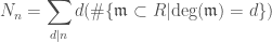
We now generalize the Riemann zeta function to any finitely generated ring \mathcal{O}_{K} with field of fractions K by writing it in the following form (this zeta function \zeta(K,s) is also called the arithmetic zeta function):

\displaystyle \zeta(K,s)=\prod_{\mathfrak{m}}\frac{1}{1-(\# \mathcal{O}_{K}/\mathfrak{m})^{-s}}

where \mathfrak{m} runs over all the maximal ideals of the ring \mathcal{O}_{K}, \mathcal{O}_{K}/\mathfrak{m} is the residue field, and the expression \#\mathcal{O}_{K}/\mathfrak{m} stands for the number of elements of this residue field. In the case that \mathcal{O}_{K}=\mathbb{Z}, we get back our usual expression for the Riemann zeta function in its Euler product form, which we have written above, since the maximal ideals of \mathbb{Z} are the principal ideals (p) generated by the prime numbers, and the residue fields \mathbb{Z}/(p) are the fields \{0,1,...,p-1\}, therefore the number \# \mathbb{Z}/(p) is equal to p.

Next we discuss finite fields. All finite fields have a number of elements equal to some positive power of a prime number p; if this number is equal to q=p^{n}, we write the finite field as \mathbb{F}_{q} or \mathbb{F}_{p^{n}}. In the case that n=1, then \mathbb{F}_{q}=\mathbb{F}_{p} is isomorphic to \mathbb{Z}/p\mathbb{Z}.

Let C be a nonsingular projective curve defined over the finite field \mathbb{F}_{q}. “Nonsingular” roughly refers to the curve being “smooth”; or “differentiable”; “projective” roughly means that the curve is part, or a subset, of some projective space. We will not be dwelling too much on these technicalities in this post. “Defined over the finite field \mathbb{F}_{q}” means that the polynomial equation that defines the curve has coefficients which are elements of the finite field \mathbb{F}_{q}. We know that in algebraic geometry (see Basics of Algebraic Geometry), the points of a curve (or more general varieties) correspond to maximal ideals of a “ring of functions” \mathcal{O}_{K} on the curve C . For a point P on a curve over a finite field \mathbb{F}_{q}, the residue field \mathcal{O}_{K}/\mathfrak{m}, where \mathfrak{m} is the maximal ideal corresponding to P, is also a finite field of the form \mathbb{F}_{q^{m}}. The number m is called the degree of P and written \text{deg}(P), and we now define another zeta function (also called the local zeta function and written Z(C,t)) via the following formula:

\displaystyle Z(C,t)=\prod_{P\in C}\frac{1}{1-t^{\text{deg}(P)}}

or equivalently,

\displaystyle Z(C,t)=\prod_{\mathfrak{m}}\frac{1}{1-t^{\text{deg}(\mathfrak{m})}}.

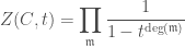
Note that this zeta function Z(C,t) is related to the other zeta function \zeta(K,s) by the following relation:

\displaystyle \zeta(K,s)=Z(C,q^{-s}).

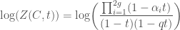
Next we take the “logarithm” of the zeta function Z(C,t). Using the familiar rules for taking the logarithms of products, we will obtain

\displaystyle \text{log}(Z(C,t))=\text{log}\bigg(\prod_{\mathfrak{m}}\frac{1}{1-t^{\text{deg}(\mathfrak{m})}}\bigg)

\displaystyle \text{log}(Z(C,t))=\sum_{\mathfrak{m}}\text{log}\bigg(\frac{1}{1-t^{\text{deg}(\mathfrak{m})}}\bigg)

\displaystyle \text{log}(Z(C,t))=-\sum_{\mathfrak{m}}\text{log}\bigg(1-t^{\text{deg}(\mathfrak{m})}\bigg)

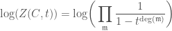
Next we will need the following series expansion for logarithms:

\displaystyle \text{log}(1-a)=-\sum_{k=0}^{\infty}\frac{a^{k}}{k}.

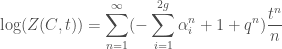
This allows us to write the logarithm of the zeta function as follows:

\displaystyle \text{log}(Z(C,t))=\sum_{\mathfrak{m}}\sum_{k=1}^{\infty}\frac{(t^{\text{deg}(\mathfrak{m})})^{k}}{k}

\displaystyle \text{log}(Z(C,t))=\sum_{\mathfrak{m}}\sum_{k=1}^{\infty}\frac{(t^{\text{deg}(\mathfrak{m})})^{k}}{k\text{deg}(\mathfrak{m})}\text{deg}(\mathfrak{m})

We can condense this expression by writing
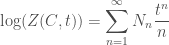
\displaystyle \text{log}(Z(C,t))=\sum_{n=1}^{\infty}N_{n}\frac{t^{n}}{n}

where

\displaystyle N_{n}=\sum_{d|n}d(\#\{\mathfrak{m}\subset R|\text{deg}(\mathfrak{m})=d\}).

The expression d|n means “n is divisible by d“, or “d divides n“, which means that the sum is taken over all d that divides n.

The numbers N_{n} can be thought of as the number of points on the curve C whose coordinates are elements of the finite field \mathbb{F}_{q^{n}}. In fact, we can actually define the zeta function Z(C,t) starting with the numbers N_{n}, i.e.

\displaystyle Z(C,t)=\text{exp}\bigg(\sum_{n=1}^{\infty}N_{n}\frac{t^{n}}{n}\bigg)

but we chose to start from the more familiar Riemann zeta function \zeta(s) and generalize to get the form we want for curves over finite fields.

We recall that the zeroes of a function f(z) are those z_{i} such that f(z_{i})=0.

We can now give the statement of the Riemann hypothesis for curves over finite fields:

The zeroes of the zeta function \zeta(K,s)=Z(C,q^{-s}) all have real part equal to \frac{1}{2}.

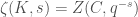
We will not discuss the entirety of Weil’s proof in this post, although the reader may consult the references provided for such a discussion. Instead we will give a rough overview of Weil’s strategy, which rests on three important assumptions. We will show, roughly, how these assumptions lead to the proof of the Riemann hypothesis, and although we will not prove the assumptions themselves, we will also give a kind of preview of the ideas involved in their respective proofs. It is these ideas, which may now be considered to have developed into entire areas of research in themselves, which are perhaps the most enduring legacy of Weil’s proof.

Assumption 1 (Rationality): The zeta function Z(C,t) can be written in the following form:

\displaystyle Z(C,t)=\frac{\prod_{i=1}^{2g}(1-\alpha_{i}t)}{(1-t)(1-qt)}

Given that this assumption holds, we can take the logarithm of the above expression,

\displaystyle \text{log}(Z(C,t))=\text{log}\bigg(\frac{\prod_{i=1}^{2g}(1-\alpha_{i}t)}{(1-t)(1-qt)}\bigg)

\displaystyle \text{log}(Z(C,t))=\sum_{i=1}^{2g}\text{log}(1-\alpha_{i}t)-\text{log}(1-t)-\text{log}(1-qt)

and we can then apply the series expansion for the logarithm that we have applied earlier to obtain the following expression,

\displaystyle \text{log}(Z(C,t))=\sum_{n=1}^{\infty}(-\sum_{i=1}^{2g}\alpha_{i}^{n}+1+q^{n})\frac{t^{n}}{n}

which we can now compare to the expression we obtained earlier for \text{log}(Z(C,t)) in terms of the number N_{n} of points with coordinates in \mathbb{F}_{q^{n}}:

\displaystyle \sum_{n=1}^{\infty}(-\sum_{i=1}^{2g}\alpha_{i}^{n}+1+q^{n})\frac{t^{n}}{n}=\sum_{n=1}^{\infty}N_{n}\frac{t^{n}}{n}.

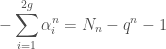
Comparing the coefficients of \frac{t^{n}}{n}, we obtain, for each n,

\displaystyle -\sum_{i=1}^{2g}\alpha_{i}^{n}+1+q^{n}=N_{n}.

With a little algebraic manipulation we have

\displaystyle -\sum_{i=1}^{2g}\alpha_{i}^{n}=N_{n}-q^{n}-1

and taking the absolute value of both sides gives us

\displaystyle |\sum_{i=1}^{2g}\alpha_{i}^{n}|=|N_{n}-q^{n}-1|

Assumption 2 (Hasse-Weil Inequality):

\displaystyle |N_{n}-q^{n}-1|\leq 2gq^{\frac{n}{2}}

This assumption, together with the earlier discussion, means that

\displaystyle |\sum_{i=1}^{2g}\alpha_{i}^{n}|\leq 2gq^{\frac{n}{2}}

We can then make use of the expansion

\displaystyle \sum_{i=1}^{2g}\frac{1}{1-\alpha_{i}(q^{-\frac{1}{2}})}=\sum_{n=1}^{\infty}(\sum_{i=1}^{2g}\alpha_{i}^{n})(q^{-\frac{1}{2}})^{n}

which in turn implies that

|\alpha_{i}|\leq q^{\frac{1}{2}}    for all i from 1 to 2g.

Assumption 3 (Functional Equation):

\displaystyle Z\bigg(C,\frac{1}{qt}\bigg)=q^{1-g}t^{2-2g}Z(C,t)

Given this assumption, and writing the zeta function Z(C,t) explicitly, we have:

\displaystyle \frac{\prod_{i=1}^{2g}(1-\alpha_{i}\frac{1}{qt})}{(1-\frac{1}{qt})(1-q\frac{1}{qt})}=q^{1-g}t^{2-2g}\frac{\prod_{i=1}^{2g}(1-\alpha_{i}t)}{(1-t)(1-qt)}

With a little algebraic manipulation we can obtain the following equation:

\displaystyle q^{g}t^{2g}\prod_{i=1}^{2g}(1-\alpha_{i}\frac{1}{qt})=\prod_{i=1}^{2g}(1-\alpha_{i}t)

Let us write the product explicitly, and make the left side zero by letting t=\frac{\alpha_{1}}{q}:

\displaystyle q^{g}(\frac{\alpha_{1}}{q})^{2g}(0)(1-\alpha_{2}\frac{1}{q}\frac{q}{\alpha_{1}})...(1-\alpha_{2g}\frac{1}{q}\frac{q}{\alpha_{1}})=(1-\alpha_{1}\frac{\alpha_{1}}{q})(1-\alpha_{2}\frac{\alpha_{1}}{q})...(1-\alpha_{2g}\frac{\alpha_{1}}{q})

Now since the left side is zero, the right side also must be zero. Therefore one of the factors in the product must be zero. This means that for some i from 1 to 2g, we have

\displaystyle 1-\alpha_{i}\frac{\alpha_{1}}{q}=0

In other words,

\displaystyle \alpha_{i}\alpha_{1}=q

This applies to any other j from 1 to 2g, not just 1, therefore more generally we must have

\displaystyle \alpha_{i}\alpha_{j}=q    for some i and j from 1 to 2g.

If we combine this result with our earlier result that

\displaystyle |\alpha_{i}|\leq q^{\frac{1}{2}}    for all i from 1 to 2g,

this means that

\displaystyle |\alpha_{i}|=q^{\frac{1}{2}}    for all i from 1 to 2g.

With this last result, we know that the zeroes of Z(C,t) must have absolute value equal to q^{-\frac{1}{2}}. Since Z(C,q^{-s})=\zeta(K,s), this implies that the real part of s must be equal to \frac{1}{2}, and this proves the Riemann hypothesis for curves over finite fields. More explicitly, let t_{0} be a zero of the zeta function Z(C,q^{-s}). We then have

\displaystyle |t_{0}|=q^{-\frac{1}{2}}

\displaystyle |q^{-s}|=q^{-\frac{1}{2}}

\displaystyle |q^{-(\text{Re}(s)+\text{Im}(s))}|=q^{-\frac{1}{2}}

\displaystyle q^{-(\text{Re}(s))}=q^{-\frac{1}{2}}

\displaystyle \text{Re}(s)=\frac{1}{2}

The proof of the rationality of the zeta function Z(C,t) and the functional equation makes use of the theory of divisors (see Divisors and the Picard Group) and a very important theorem in algebraic geometry called the Riemann-Roch theorem. The Riemann-Roch theorem originates from complex analysis, which was the kind of the “specialty” of Bernhard Riemann (“On the Number of Primes Less Than a Given Magnitude” was his only paper on number theory, and it concerns the application of complex analysis to number theory). In its original formulation, the Riemann-Roch theorem gives the dimension of the vector space formed by the functions whose zeroes and poles (for a function which can be expressed as the ratio of two polynomials, the poles can be thought of as the zeroes of the denominator), and their “order of vanishing”, are specified. The Riemann-Roch theorem has since been generalized to aspects of algebraic geometry not necessarily directly concerned with complex analysis, and it is this generalization that allows us to make use of it for the case at hand.

In addition to the theory of divisors and the Riemann-Roch theorem, to prove the Hasse-Weil inequality, one must make use of the theory of fixed points, applied to what is known as the Frobenius morphism, which sends a point of C with coordinates a_{i} to the point with coordinates a_{i}^{q}. The theory of fixed points is related to the part of algebraic geometry known as intersection theory. Roughly, given a function f(x), we can think of its fixed points as the values of x for which f(x)=x. One way to obtain these fixed points is to draw the graph of y=x, and the graph of y=f(x), on the xy plane; the fixed points of f(x) are then given by the points where the two graphs intersect.

For the Frobenius morphism, the fixed points correspond to those points whose coordinates are elements of the finite field \mathbb{F}_{q}. Similarly, the fixed points of the n-th power of the Frobenius morphism (which we can think of as the Frobenius morphism applied n times) correspond to those points whose coordinates are elements of the finite field \mathbb{F}_{q^{n}}. Hence we can obtain the numbers N_{n} that go into the expression of the zeta function Z(C,t) using the Frobenius morphism. Combined with results from intersection theory such as the Castelnuovo-Severi inequality and the Hodge index theorem, this allows us to prove the Hasse-Weil inequality.

In algebraic geometry, curves are one-dimensional varieties, and just as there is a version of the Riemann hypothesis for curves over finite fields, there is also a version of the Riemann hypothesis for higher-dimensional varieties over finite fields, called the Weil conjectures, since they were proposed by Weil himself after he proved the case for curves. The Weil conjectures themselves follow the important assumptions involved in proving the Riemann hypothesis for curves over finite fields, such as the rationality of the zeta function and the functional equation. In addition, part of the Weil conjectures suggests a connection with the theory of cohomology (see Homology and Cohomology and Cohomology in Algebraic Geometry), which significant implications for the connections between algebraic geometry and methods originally developed for algebraic topology.

The Weil conjectures were proved by Bernard Dwork, Alexander Grothendieck, and Pierre Deligne. In his efforts to prove the Weil conjectures, Grothendieck developed the notion of topos (see More Category Theory: The Grothendieck Topos), as well as etale cohomology. As further part of his approach, Grothendieck also proposed conjectures, known as the standard conjectures on algebraic cycles, which remain open to this day. Grothendieck’s student, Pierre Deligne, was able to complete the proof of the Weil conjectures while bypassing the standard conjectures on algebraic cycles, by developing ingenious methods of his own. Still, the standard conjectures on algebraic cycles, as well as the related theory of motives, remain very much interesting on their own and continue to be a subject of modern mathematical research.

References:

Riemann Hypothesis on Wikipedia

Weil Conjectures on Wikipedia

Arithmetic Zeta Function on Wikipedia

Local Zeta Function on Wikipedia

The Weil Conjectures for Curves by Sam Raskin

Algebraic Geometry by Bas Edixhoven and Lenny Taelman

The Riemann Hypothesis over Finite Fields: From Weil to the Present Day by J.S. Milne

Algebraic Geometry by Robin Hartshorne