We have discussed elliptic curves over the rational numbers, the real numbers, and the complex numbers in Elliptic Curves. In this post, we discuss elliptic curves over finite fields of the form 

We recall that in Elliptic Curves we gave the definition of an elliptic curve as a polynomial equation that we may write as

with 


Still, we claimed that we will not be able to write the equation of the elliptic curve when the coefficients of the elliptic curve are of characteristic equal to 


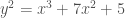
Let both 

whose graph in the 


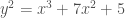
Next let 


and whose graph is given by the following figure (again plotted using WolframAlpha):

Note also that in both cases, the right hand side of the equations of the curves are polynomials in 


The two curves,
We now introduce the general form of an elliptic curve, applicable even when the coefficients belong to fields of characteristic 


This equation is called the long Weierstrass equation. We may also say that it is in long Weierstrass form.
We can now define what it means for a curve to be singular. Let

Then a singular point on this curve 


It might be difficult to think of calculus when we are considering, for example, curves over finite fields, where there are a finite number of points on the curve, so we might instead just think of the partial derivatives of the curve as being obtained “algebraically” using the “power rule” of basic calculus,

and applying it, along with the usual rules for partial derivatives and constant factors, to every term of the curve. Such is the power of algebraic geometry; it allows us to “import” techniques from calculus and other areas of mathematics which we would not ordinarily think of as being applicable to cases such as curves over finite fields.
If a curve has no singular points, then it is called a nonsingular curve. We may also say that the curve is smooth. In order for a curve written in long Weierstrass form to be an elliptic curve, we require that it be a nonsingular curve as well.
If the coefficients of the curve are not of characteristic equal to

In this case the condition for the curve to be nonsingular can be written in the following form:

The quantity

is called the discriminant of the curve.
We note now, of course, that the usual expressions for the elliptic curve, in what we call affine coordinates 


We now consider an elliptic curve whose equation has coefficients which are rational numbers. We can make a projective transformation of variables to rewrite the equation into one which has integers as coefficients. Then we can reduce the coefficients modulo a prime
It may happen that when we reduce an elliptic curve modulo

Let us reduce this modulo the prime 


over 


In the case that an elliptic curve has bad reduction at
As we have already seen in The Riemann Hypothesis for Curves over Finite Fields, whenever we have a curve over some finite field 


We can now define the Hasse-Weil L-function of an elliptic curve 
where


The Hasse-Weil L-function encodes number-theoretic information related to the elliptic curve, and much of modern mathematical research involves this function. For example, the Birch and Swinnerton-Dyer conjecture says that the rank of the group formed by the rational points of the elliptic curve (see Elliptic Curves), also known as the Mordell-Weil group, is equal to the order of the zero of the Hasse-Weil L-function at 

where 
Meanwhile, the Shimura-Taniyama-Weil conjecture, now also known as the modularity conjecture, central to Andrew Wiles’s proof of Fermat’s Last Theorem, states that the Hasse-Weil L-function can be expressed as the following series:

and the coefficients 


For more on the modularity theorem and Wiles’s proof of Fermat’s Last Theorem, the reader is encouraged to read the award-winning article A Marvelous Proof by Fernando Q. Gouvea, which is freely and legally available online. A link to this article (hosted on the website of the Mathematical Association of America) is provided among the list of references below.
References:
Hasse-Weil Zeta Function on Wikipedia
Birch and Swinnerton-Dyer Conjecture on Wikipedia
Modularity Theorem on Wikipedia
Wiles’s Proof of Fermat’s Last Theorem on Wikipedia
The Birch and Swinnerton-Dyer Conjecture by Andrew Wiles
A Marvelous Proof by Fernando Q. Gouvea
A Friendly Introduction to Number Theory by Joseph H. Silverman
The Arithmetic of Elliptic Curves by Joseph H. Silverman
Advanced Topics in the Arithmetic of Elliptic Curves by Joseph H. Silverman
Invitation to the Mathematics of Fermat-Wiles by Yves Hellegouarch
A First Course in Modular Forms by Fred Diamond and Jerry Shurman

Pingback: Algebraic Cycles and Intersection Theory | Theories and Theorems
Pingback: SEAMS School Manila 2017: Topics on Elliptic Curves | Theories and Theorems