Hilbert Modular Surfaces

June 8, 2023February 14, 2024 / Anton Hilado / Leave a comment

Hilbert Modular Surfaces and Hilbert Modular Forms: The Basics

A Hilbert modular surface is a kind of Shimura variety (see Shimura Varieties), in a sense one of the next simplest after modular curves (although Shimura curves have lower dimension and Siegel modular threefolds have a simpler moduli interpretation). Aside from being a higher-dimensional analogue of modular curves, Hilbert modular surfaces possess interesting structure not present in modular curves. For example, Hilbert modular forms may contain embedded modular curves as codimension $1$ subvarieties!

We begin with the definition. Let $F=\mathbb{Q}(\sqrt{d})$ , where $d$ is a squarefree positive integer, i.e. $F$ is a real quadratic field. We denote its ring of integers by $\mathcal{O}_{F}$ . The group $\Gamma=\mathrm{SL}_{2}(\mathcal{O}_{F})$ acts on the product $\mathbb{H}\times \mathbb{H}$ of two upper half-planes as follows:

$\displaystyle \begin{pmatrix} a & b \\ c & d \end{pmatrix}(z_{1},z_{2})=\left(\frac{az_{1}+b}{cz_{1}+d},\frac{a'z_{2}+b'}{c'z_{2}+d'}\right)$

for $(z_{1},z_{2})\in \mathbb{H}\times\mathbb{H}$ , where $a',b',c',d'$ are the Galois conjugates of $a,b,c,d$ . If we then take the left quotient of $\mathbb{H}\times\mathbb{H}$ by this action of $\Gamma)$ , we then end up with a complex analytic surface $Y(\Gamma)$ , which is non-compact. Just as the “open” modular curve constructed in The Moduli Space of Elliptic Curves parametrizes elliptic curves over $\mathbb{C}$ , the open modular surface $Y(\Gamma)$ which we have just constructed parametrizes abelian surfaces $A$ over $\mathbb{C}$ with an extra “real multiplication” structure, which is an embedding of $\mathcal{O}_{F}$ into their ring of endomorphisms $\mathrm{End}(A)$ .

We may “compactify” the above construction by instead considering the quotient $\Gamma\backslash(\mathbb{H}\times\mathbb{H}\cup\mathbb{P}^1(F))$ (note that $\mathbb{P}^{1}(F)$ is also equipped with an action of $\Gamma$ ), which adds a finite number (equal to the class number of $F$ ) of points called cusps. This compactification, which we denote $X(\Gamma)$ , will be singular. However, by the theory developed by Heisuke Hironaka, there is a way to “resolve” the singularities, and by applying this theory we may obtain a smooth projective surface $\widetilde{X}(\Gamma)$ .

Hilbert modular surfaces are the natural home of Hilbert modular forms (although Hilbert modular forms live on Hilbert modular varieties, more generally, as we mention in the next paragraph). A Hilbert modular form of weight $(k_{1},k_{2})$ is a meromorphic function $f$ on $\mathbb{H}\times\mathbb{H}$ such that, for $\gamma=\begin{pmatrix}a & b \\ c & d\end{pmatrix}\in\Gamma$ , we have

$\displaystyle f(\gamma z)=(cz_{1}+d)^{k_{1}}(c'z_{2}+d')^{k_{2}}f(z_{1},z_{2})$

From the point of view of algebraic geometry, Hilbert modular forms can also be obtained as sections of certain sheaves on a Hilbert modular surface.

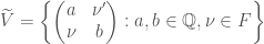
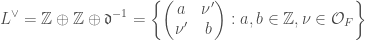
Before we continue our discussion of Hilbert modular surfaces, we note that all of the above constructions may be generalized by letting $F$ be a more general totally real field, instead of just a real quadratic field. This leads to the more general notion of a Hilbert modular variety, and of more general Hilbert modular forms. We also note that instead of $\Gamma=\mathrm{SL}_{2}(\mathcal{O}_{F})$ , we could instead consider some nontrivial level structure $\Gamma=\Gamma(\mathcal{O}_{F}\oplus\mathfrak{a})$ , where $\mathfrak{a}$ is some fractional ideal of $\mathcal{O}_{F}$ . The group $\Gamma(\mathcal{O}_{F}\oplus\mathfrak{a})$ is defined to be the group of matrices of the form $\begin{pmatrix} a & b \\ c & d \end{pmatrix}$ where $a,d\in\mathcal{O}_{F}$ , $b\in\mathfrak{a}^{-1}$ , and $c\in\mathfrak{a}$ .

A Whirlwind Introduction to Clifford Algebras and Spin Groups

We have so far described Hilbert modular surfaces and Hilbert modular forms in terms of the group $\mathrm{SL}_{2}(F)$ . However there is another way to describe them via the exceptional isomorphisms of spin groups (which are double covers of special orthogonal groups, see also Rotations in Three Dimensions) with other groups – In our case, we have the isomorphism $\mathrm{Spin}(2,2)\simeq\mathrm{SL}_{2}(F)$ . Let us discuss first the general theory behind spin groups of signature $(2,n)$ and their associated symmetric spaces, and then later we apply it to the specific case of Hilbert modular surfaces.

Let $(V,q)$ be a pair consisting of a vector space $V$ over $\mathbb{Q}$ and a quadratic form $q$ . The orthogonal group $\mathrm{O}(V)$ is the subgroup of the group of linear transformations of $V$ which preserve $q$ . The Clifford algebra $C_{V}$ associated to $(V,q)$ is the quotient of the tensor algebra of $V$ by the relation, for all $v\in V$ ,

$\displaystyle v^{2}=q(v)$

The Clifford algebra generalizes many familiar constructions such as the complex numbers (for $V=\mathbb{R}$ and $q(v)=-v^{2}$ ) and Hamilton’s quaternions for $V=\mathbb{R}^{2}$ and $q(v_{1}+v_{2})=-v_{1}^{2}-v_{2}^{2}$ . Note that, unlike the complex numbers, more general Clifford algebras such as Hamilton’s quaternions have more than one type of “conjugation”. The first, which we shall call $J$ , is induced by negation of basis elements of $V$ . Another is given by cyclically permuting the tensor factors of an element so that $x^{t}=v_{2}\otimes\ldots \otimes v_{m}\otimes v_{1}$ for $v=v_{1}\otimes\ldots\otimes v_{m}$ . This second conjugation allows us to define the Clifford norm:

$\displaystyle \mathrm{Nm}(v)=v^{t}v$

The even Clifford algebra $C_{V}^{0}$ of $C_{V}$ is the subalgebra generated by elements which are a product of an even number of basis elements of $V$ . The odd part $C_{V}^{1}$ is similarly defined, and we have the decomposition $C_{V}=C_{V}^{0}\oplus C_{V}^{1}$ . The Clifford group is defined to be the set of all invertible elements $v$ of the Clifford algebra such that $vVJ(v)^{-1}=V$ . The intersection of the even Clifford algebra and the Clifford group is called $\mathrm{GSpin}(V)$ . The set of elements of $\mathrm{GSpin}(V)$ whose Clifford norm is equal to $1$ is called $\mathrm{Spin}(V)$ .

We now mention some facts about the special case when $V$ has dimension $4$ that we will use later when we discuss Hilbert modular surfaces again. Let $v_{1},v_{2},v_{3},v_{4}$ be a basis of $V$ such that $q(v_{i})\neq 0$ for all $i$ . Let $\delta=v_{1}v_{2}v_{3}v_{4}$ . The center $Z$ of the Clifford algebra associated to $(V,q)$ is then isomorphic to $\mathbb{Q}+\mathbb{Q}\delta$ , and the even Clifford algebra admits the description

$\displaystyle C_{V}^{0}=Z+Zv_{1}v_{2}+Zv_{2}v_{3}+Zv_{1}v_{3}$

Fix an element $v_{0}\in V$ such that $q(v_{0})\neq 0$ and for $v\in C_{V}^{0}$ let $v^{\sigma}=v_{0}vv_{0}^{-1}$ . We define the new vector space $\widetilde{V}$ to be the set of all elements $v$ of $C_{V}^{0}$ such that the automorphism $v^{\sigma}$ agrees with the conjugation $v^{t}$ , and we equip $\widetilde{V}$ with the quadratic form $\widetilde{q}(v)=q(v_{0})\cdot \mathrm{Nm}(v)$ . It turns out that $(\widetilde{V},\widetilde{q})$ is isometric to $(V,q)$ , and the upshot is that we can now describe the action of an element $g\in\mathrm{Spin}(V)$ on an element $v\in\widetilde{V}$ as follows:

$\displaystyle g(v)=gVg^{-\sigma}$ .

Symmetric Spaces for Orthogonal Groups of Signature (2,n): Three Descriptions

The upper-half plane is the “symmetric space” for the group $\mathrm{SL}_{2}(\mathbb{R})$ , and may be obtained as the quotient of $\mathrm{SL}_{2}(\mathbb{R})$ by its locally compact subgroup $\mathrm{SO}(2)$ . We want to generalize this to the group $\mathrm{O}(V)$ , but it is often useful to have different descriptions of the symmetric space. We will discuss three different descriptions of the symmetric space on which $\mathrm{O}(V)$ acts, each one with its own advantages and disadvantages.

First we give the “Grassmannian model“. The Grassmannian parametrizes $k$ -dimensional subspaces of a vector space. It is a generalization of projective space (which is the special case when $k=1$ ). In our case, we want to parametrize $2$ -dimensional spaces of $V$ , with the additional condition that the quadratic form $q$ is positive definite on this space:

$\displaystyle \mathrm{Gr}(V)=\lbrace v\in V:\mathrm{dim}(v)=2\mbox{ and }q\vert_{v}>0\rbrace$

The group $\mathrm{O}(V)$ acts on $\mathrm{Gr}(V)$ , and the stabilizer of an element $v_{0}$ is a maximal compact subgroup $K$ , which is isomorphic to $\mathrm{O}(2)\times \mathrm{O}(n)$ . Therefore we can see that $\mathrm{Gr}(V)\cong \mathrm{O}(V)/K$ , and provides a realization of its associated symmetric space. However, in this model it is harder to see the complex analytic structure.

This problem can be remedied by considering the “projective model“. Let $V(\mathbb{C})$ be the complexification of $V$ and define

$\displaystyle \mathcal{K}=\lbrace[z]\in\mathbb{P}(V(\mathbb{C})):(z,z)=0,(z,\overline{z})>0\rbrace$

Now $\mathcal{K}$ is an $n$ -dimensional complex manifold consisting of two connected components. We choose one of these components and denote it by $\mathcal{K}^{+}$ – this is our symmetric space. Although the complex analytic structure is easier to see in the projective model, it is hard to relate this model to well-known examples of symmetric spaces such as the upper half-plane (which is the case when $n=1$ ).

Finally we consider the “tube domain model“. Let $e_{1}$ be a nonzero isotropic vector in $V$ and let $e_{2}$ be another vector in $V$ such that $(e_{1},e_{2})=1$ . We let $W$ be the intersection of the orthogonal complements of $e_{1}$ and $e_{2}$ in $V$ , so that

$\displaystyle V=W\oplus \mathbb{C}e_{1}\oplus\mathbb{C}e_{2}$

On the vector space $W$ , the restriction of the quadratic form $q$ has signature $1,n-1$ . We let $W(\mathbb{C})$ denote the complexification of $W$ and define

$\displaystyle \mathcal{H}=\lbrace z\in W(\mathbb{C}):q(\mathrm{Im}(z))>0)\rbrace$

We can define a biholomorphic map between $\mathcal{H}$ and $\mathcal{K}$ by sending $z$ to $[(z,1,-q(z)-q(e_{2}))]$ . We denote the preimage of $\mathcal{K}^{+}$ by $\mathcal{H}^{+}$ – the latter is analogous to the upper half-plane.

Heegner Divisors

Let us now consider smaller modular varieties embedded in other bigger modular varieties. Let $L$ be a lattice in $V$ . The idea is that if we pick a vector $\lambda$ in the dual lattice $L^{\vee}$ in $V$ , and consider the orthogonal complement of $\lambda$ in $V$ , what we get is actually a vector space of signature $2,n-1$ , to which we can once again apply the preceding constructions! Applied to the case of Hilbert modular surfaces, this explains the embedded modular curves. In symbols, we have

$\displaystyle H_{\lambda}=\lbrace [Z]\in\mathcal{K}^{+}:(Z,\lambda)=0\rbrace$

If we write $\lambda=\lambda_{W}+ae_{2}+be_{1}$ , then we can also describe $H_{\lambda}$ in the tube domain model as follows:

$\displaystyle H_{\lambda}=\lbrace z\in\mathcal{H}^{+}:aq(z)-(z,\lambda_{W})-aq(e_{2})-b=0\rbrace$

We can now define the Heegner divisor $H(\beta,m)$ as the sum of all the $H_{\lambda}$ where $\lambda\in\beta+L$ satisfies the condition that $q(\lambda)=m$ . We can further define the composite Heegner divisor $H(m)$ as half the sum of all Heegner divisors $H(\beta,m)$ as $\beta$ runs over $L^{\vee}/L$ .

Back to Hilbert Modular Surfaces

We now go back to our setting of Hilbert modular surfaces and apply the above theory to the $4$ -dimensional vector space $V=\mathbb{Q}\oplus\mathbb{Q}\oplus F$ , equipped with the quadratic form $q(a,b,\nu)=\nu\nu'-ab$ . We choose the following basis for $V$ :

$\displaystyle v_{1}=(1,1,0)$

$\displaystyle v_{2}=(1,-1,0)$

$\displaystyle v_{3}=(0,0,1)$

$\displaystyle v_{4}=(0,0,\sqrt{d})$

In this case the center of the Clifford algebra is isomorphic to $F$ , and the even Clifford algebra $C_{V}^{0}$ of $V$ is of the form $C_{V}^{0}=F+Fv_{1}v_{2}+Fv_{2}v_{3}+Fv_{1}v_{3}$ . Via the assignments

$\displaystyle 1\mapsto\begin{pmatrix}1 & 0 \\ 0 & 1\end{pmatrix}$

$\displaystyle v_{1}v_{2}\mapsto\begin{pmatrix}1 & 0 \\ 0 & -1\end{pmatrix}$

$\displaystyle v_{2}v_{3}\mapsto\begin{pmatrix}0 & 1 \\ -1 & 0\end{pmatrix}$

$\displaystyle v_{1}v_{3}\mapsto\begin{pmatrix}0 & 1 \\ 1 & 0\end{pmatrix}$

we have an isomorphism between $C_{V}^{0}$ and $M_{2}(F)$ . Furthermore, the Clifford norm on $C_{V}^{0}$ corresponds to the determinant on $M_{2}(F)$ . All in all, this gives us an isomorphism between $\mathrm{Spin}_{V}$ and $\mathrm{SL}_{2}(F)$ . The theory we have discussed earlier provides us with the following vector space $\widetilde{V}$ isomorphic to $V$ :

$\displaystyle \widetilde{V}=\left\lbrace \begin{pmatrix} a & \nu' \\ \nu & b\end{pmatrix}:a,b\in\mathbb{Q},\nu\in F\right\rbrace$

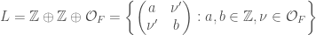
We also have a description of the lattices $L$ and $L^{\vee}$ as matrices inside $\widetilde{V}$ as follows:

$\displaystyle L=\mathbb{Z}\oplus\mathbb{Z}\oplus\mathcal{O}_{F}=\left\lbrace\begin{pmatrix}a & \nu' \\ \nu' & b\end{pmatrix}:a,b\in\mathbb{Z},\nu\in\mathcal{O}_{F}\right\rbrace$

$\displaystyle L^{\vee}=\mathbb{Z}\oplus\mathbb{Z}\oplus\mathfrak{d}^{-1}=\left\lbrace\begin{pmatrix}a & \nu' \\ \nu' & b\end{pmatrix}:a,b\in\mathbb{Z},\nu\in\mathcal{O}_{F}\right\rbrace$

It turns out, just as we have 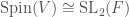$\mathrm{Spin}(V)\cong \mathrm{SL}_{2}(F)$ , we also have 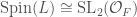$\mathrm{Spin}(L)\cong\mathrm{SL}_{2}(\mathcal{O}_{F})$ . In turn this gives us an isomorphism $Y(\Gamma)\cong Y(\mathrm{Spin}(L))$ .

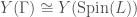Now we apply the general theory of Heegner divisors. In the special case of Hilbert modular surfaces, the Heegner divisors $H(-m/D)$ where $D$ is the discriminant of $F$ are also known as Hirzebruch-Zagier divisors. They have the explicit description

$\displaystyle T_{m}=\sum\lbrace(z_{1},z_{2}\in\mathbb{H}\times\mathbb{H}):az_{1}z_{2}+\lambda z_{1}+\lambda' z_{2}+b\rbrace$

where the sum is over all $(a,b,\lambda)\in L^{\vee}/\lbrace\pm 1\rbrace$ such that $ab-\lambda\lambda'=m$ . As a special case, $T_{1}$ is the modular curve of level $1$ (i.e. the compactified moduli space of elliptic curves).

Borcherds Products and the Kudla Program: A Preview

Hirzebruch-Zagier divisors are related to certain Hilbert modular forms called Borcherds products, which arise as “theta lifts” (see also The Theta Correspondence) of weakly holomorphic modular forms (which are almost the same as modular forms, but the holomorphicity condition at the cusps is relaxed). Here “theta lifts” is in quotes because the liftings are somewhat different from what is described in The Theta Correspondence; for one, the integral is divergent and requires a “regularization” to get it to converge, and the lifting is multiplicative, which gives it an expression as an infinite product – hence the name “Borcherds products”.

The Hirzebruch-Zagier divisors, or more generally the Heegner divisors, or even more generally “special cycles” can also be put together in a certain way to form a generating series, which should form a “modular form valued in the Chow group”. This is part of what is known as the “Kudla program” which has applications for instance to conjectures on special values of L-functions (which generalize the Birch and Swinnerton-Dyer conjecture). These and other fascinating aspects of orthogonal and unitary Shimura varieties will hopefully be covered in future posts.

References:

Hilbert modular variety on Wikipedia

Hilbert modular form on Wikipedia

Hilbert modular forms and their applications by Jan Hendrik Bruinier

Hilbert Modular Surfaces by Gerard van der Geer

The 1-2-3 of Modular Forms by Jan Hendrik Bruinier, Gunter Harder, Gerard van der Geer, and Don Zagier

Prismatic Cohomology: An Overview

May 8, 2023May 15, 2023 / Anton Hilado / 1 Comment

In p-adic Hodge Theory: An Overview, we discussed how the different cohomologies of some smooth projective variety over the p-adic numbers (or some finite extension of it) such as its p-adic etale cohomology, de Rham cohomology, or crystalline cohomology can be related to each other via the machinery of period rings.

We note that the theories we have discussed in p-adic Hodge Theory: An Overview are “rational”, in that they involve cohomologies with “rational” coefficients (for instance $H_{\mathrm{et}}^{1}(X,\mathbb{Q}_{\ell})$ ). Cohomology with integral coefficients holds some information that gets lost when passing to rational coefficients; for instance, all the information about the torsion is lost. If we want to relate, say, torsion subgroups of different cohomologies to each other, we would need some sort of integral p-adic Hodge theory. In this post, we will discuss one approach to integral p-adic Hodge theory, called prismatic cohomology, developed by Bhargav Bhatt and Peter Scholze.

As a preliminary to defining prismatic cohomology, we briefly discuss the concept of $\delta$ -rings. A $\delta$ -ring is a ring $R$ together with a map $\delta:R\to R$ called a p-derivation, satisfying the following properties:

$\displaystyle \delta(xy)=\delta(x)+\delta(y)+\frac{x^{p}+y^{p}-(x+y)^{p}}{p}$

$\displaystyle \delta(xy)=x^{p}\delta(y)+y^{p}\delta(x)+p\delta(y)\delta(x)$

$\displaystyle \delta(1)=\delta(0)=0$

The concept of $\delta$ -rings were introduced by Andre Joyal, and its theory and that of p-derivations was further developed by Alexandru Buium. This also has connections to the work of James Borger as we discussed in The Field with One Element.

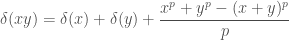
A prism is a pair $(A,I)$ consisting of a $\delta$ -ring $A$ an ideal $I$ defining a Cartier divisor on $\mathrm{Spec}(A)$ , such that $A$ is derived $(p,I)$ -complete (this means that for every $f\in(p,I)$ we have, considering $A$ as a module over itself, $\mathrm{Hom}(A_{f},A)=0$ and $\mathrm{Ext}_{A}^{1}(A_{f},A)=0$ ) and $p\in I+\phi(I)A$ .

An example of a prism is given by taking $A=\mathbb{Z}_{p}[[u]]$ and taking $I=(u-p)$ . Another important example that we will show up again later in this post is given by $A=A_{\mathrm{inf}}(\mathcal{O}_{\mathbb{C}_{p}})$ and $I=\mathrm{ker}(\theta)$ , where $\theta:A_{\mathrm{inf}}(\mathcal{O}_{\mathbb{C}_{p}})\to \mathcal{O}_{\mathbb{C}_{p}}$ is the canonical map (see also Perfectoid Fields for a discussion of these concepts).

Prisms are also related to (integral) perfectoid rings (see also Adic Spaces and Perfectoid Spaces). A prism $(A,I)$ is perfect if the ring $A$ is perfect (i.e. the Frobenius is an automorphism). If $(A,I)$ is a perfect prism, then the quotient $A/I$ is an perfectoid ring. In fact, there is an equivalence of categories between perfect prisms and perfectoid rings, and one can go the other way via the $A_{\mathrm{inf}}$ construction, i.e. given a perfectoid ring $R$ we set $A=W(R^{\flat})$ , and there is a canonical map $\theta:W(R^{\flat})\to R$ , and we set $I=\mathrm{ker}({\theta})$ ; then the pair $(A,I)$ obtained via this construction is a prism.

Remark: The perfectoid rings mentioned in the previous paragraph are related, but not quite the same, as in Adic Spaces and Perfectoid Spaces. The perfectoid rings in the previous paragraph and in the rest of the article correspond to the ring of integral elements of the perfectoid rings in Adic Spaces and Perfectoid Spaces, hence the word “integral”. To match with the references, we will drop the word “integral” in the rest of this post, but perfectoid rings in this post will mean integral perfectoid rings.

Let $(A,I)$ be a prism and let $R$ be a formally smooth $A/I$ -algebra. The prismatic site of $R$ relative to $A$ , denoted $(R/A)_{\Delta}$ , is the category of prisms $(B, IB)$ over $A$ together with a map from $R$ to $B/IB$ over $A$ . We write such an object as $(R\rightarrow B/IB\leftarrow B)$ . We have functors $\mathcal{O}_{\Delta}$ and $\overline{\mathcal{O}}_{\Delta}$ which send $(R\rightarrow B/IB\leftarrow B)$ to $B$ and $B/IB$ respectively. We now define the prismatic cohomology of $R$ , denoted $\Delta_{R/A}$ , to be $R\Gamma((R/A)_{\Delta},\mathcal{O})$ . As an example, in the special case that $R=A/I$ , then the prismatic cohomology $\Delta_{R/A}$ is just $A$ .

Related to prisms and prismatic cohomology is the notion of prismatic crystals. A prismatic crystal is an assignment, given a prism $(B,J)$ in $\Delta_{R/A}$ , of a finite projective $B$ -module. We also have related notions of Hodge-Tate crystals (which assign finite projective $B/J$ -modules instead), prismatic F-crystals (prismatic crystals $\mathcal{E}$ with an isomorphism $\phi^{*}\mathcal{E}[1/I]\to\mathcal{E}[1/I]$ ), and notions of crystals where instead of modules we consider complexes (perfect or $(p,I)$ -complete) of modules.

The prismatic cohomology $\Delta_{R/A}$ is equipped with some other extra structures, for instance we have the notion of a Breuil-Kisin twist $\Delta_{R/A}\{ 1\}$ , which corresponds to the Tate twist in etale cohomology. The prismatic cohomology also comes with a filtration, called the Nygaard filtration. These structures are important for some of the applications of prismatic cohomology. For instance, the two notions just discussed allows us to give a definition of syntomic cohomology as follows:

$\displaystyle \mathbb{Z}_{p}(i)(R)=\mathrm{fib}(\mathrm{Fil}^{i}\Delta_{R/A}\{i\}\xrightarrow{\phi_{i}-1}\Delta_{R/A}\{i\})$

The syntomic cohomology is related to etale K-theory of p-adically complete rings; in particular, there is a motivic filtration on the etale K-theory whose graded pieces are given by shifts of the syntomic cohomology. This relation between etale K-theory and syntomic cohomology goes through the theory of topological cyclic homology (and other related theories such as topological Hochschild homology) and hints at deep connections between prismatic cohomology and algebraic topology; we leave further discussion of these directions to the references or possible future posts.

As mentioned earlier, prismatic cohomology gives us an integral version of p-adic Hodge theory. Therefore, it must be related to the different cohomology theories such as crystalline cohomology and etale cohomology. This relationship is explicitly stated in the form of the following comparison theorems. For crystalline cohomology, we have (in the language of derived categories)

$\displaystyle R\Gamma_{\mathrm{crys}}(R/A)\cong \phi_{A}^{*}\Delta_{R/A}$

The crystalline cohomology can be considered a “lift” of the de Rham cohomology; namely the de Rham complex $\Omega_{R/(A/p)}^{\bullet}$ that computes the de Rham cohomology of $R$ over $A/(p)$ is related to $R\Gamma_{\mathrm{crys}}(R/A)$ as follows:

$\displaystyle R\Gamma_{\mathrm{crys}}(R/A)\otimes_{A}^{\mathbb{L}}A/p=\Omega_{R/(A/p)}^{\bullet}$

And so we see that prismatic cohomology also computes de Rham cohomology. Meanwhile, for etale cohomology, letting $d$ be an element of $A$ such that $\delta(d)\in A^{\times}$ (we call such an element $d$ a distinguished element), we have

$\displaystyle R\Gamma_{\mathrm{et}}(\mathrm{Spec}(R)[1/p],\mathbb{Z}/p^{n})\cong (\Delta_{R/A}[1/d]/p^{n})^{\phi=1}$

These comparison theorems of prismatic cohomology can be used to obtain results regarding cohomology with torsion coefficients. For instance, let $X$ be a proper formal scheme over $\mathcal{O}_{\mathbb{C}_{p}}$ . Let $(A,I)$ be the prism given by $A=A_{\mathrm{inf}}(\mathcal{O}_{\mathbb{C}_{p}})$ and $I=\mathrm{ker}(\theta)$ . Then one can construct the prismatic cohomology $\Delta_{X/A}$ by gluing together the different $\Delta_{R/A}$ for every $\mathrm{Spf}(R)\subset X$ , and then use the comparison theorems previously mentioned to prove the following result:

$\displaystyle \mathrm{dim}_{\mathbb{F}_{p}}H^{i}(X^{\mathrm{an}},\mathbb{Z}/p)\leq\mathrm{dim}_{\mathbb{F}_{p}}H_{\mathrm{dR}}^{i}(X)$

Note that this result involves torsion coefficients, and therefore inaccessible if one does not have an “integral” p-adic Hodge theory.

Another application of ideas from prismatic cohomology is the construction of a p-adic Riemann-Hilbert correspondence by Bhargav Bhatt and Jacob Lurie. The classical Riemann-Hilbert correspondence is an equivalence of derived categories between regular holonomic D-modules and Zariski constructible sheaves, itself an upgrade of a classical equivalence of categories between algebraic vector bundles with regular flat connection (which we may think of as differential equations) and local systems of complex vector spaces (which we may think of as solutions to these differential equations) on a smooth complex algebraic variety.

Bhatt and Lurie have developed a version of the Riemann-Hilbert correspondence for perfectoid spaces, making use of perfected prismatic cohomology, and the way it allows us to construct a “perfectoidization” of a ring. Given any ring, its perfectoidization is an $R$ -algebra $R_{\mathrm{pfd}}$ which is perfectoid, and such that for any other perfectoid ring $S$ , $\mathrm{Hom}(R_{\mathrm{pfd}},S)\cong \mathrm{Hom}(R,S)$ . As we just stated, a way to construct the perfectoidization is given by the perfected prismatic cohomology. Let $R=A/I$ be perfectoid. We define the following complex:

$\displaystyle \Delta_{R/A,\mathrm{perf}}=\varinjlim(\Delta_{R/A}\xrightarrow{\phi}\Delta_{R/A}\xrightarrow{\phi}\ldots)^{\wedge}$

Now let $S$ be a finite $R$ -algebra, and $Y=\mathrm{Spec}(S)$ . The pair $(H_{\Delta,\mathrm{perf}}^{0}(Y),IH_{\Delta,\mathrm{perf}}^{0}(Y))$ is a perfect prism, and the quotient $H_{\Delta,\mathrm{perf}}^{0}(Y)/I$ is a perfectoidization of $S$ (which we may therefore also denote by $S_{\mathrm{pfd}}$ ).

Let $f:U\to X$ be an etale morphism. We may express this as the composition $U\xrightarrow{j}\overline{U}\xrightarrow{\overline{f}}X$ , where $\overline{f}$ is finite. We may express $\overline{U}=\mathrm{Spec}(S)$ and $\overline{U}=\mathrm{S/J}$ . Then we can define

$\displaystyle \overline{\Gamma}_{c}(U)=\mathrm{ker}(S_{\mathrm{pfd}}\twoheadrightarrow (S/J)_{\mathrm{pfd}})$

If $R$ is a perfect $\mathbb{F}_{p}$ -algebra, then the functor which sends the sheaf $f_{!}\underline{\mathbb{F}_{p}}$ to $\overline{\Gamma}_{c}(U)$ may be taken to be a Riemann-Hilbert functor, agreeing with previous constructions of Bhatt and Lurie. Inspired by this, in the more general case we can define

$\displaystyle \Gamma_{c}(U)=\mathrm{ker}(H_{\Delta,\mathrm{perf}}^{0}(\overline{U})\twoheadrightarrow H_{\Delta,\mathrm{perf}}^{0}(\partial\overline{U}))$

Note that $\Gamma_{c}(U)$ is an $A$ -module, and that $\overline{\Gamma}_{c}(U)=R\otimes_{A}\Gamma_{c}(U)$ . For an etale morphism $f:U\to X$ , let $h_{U}$ be the sheaf $f_{!}\underline{\mathbb{Z}}$ on $X_{\mathrm{et}}$ , where $\underline{\mathbb{Z}}$ is the constant sheaf of $\mathbb{Z}$ -coefficients. Sheaves of this form generate the category of abelian sheaves on $X_{\mathrm{et}}$ . The Riemann-Hilbert functor for perfectoid spaces is then the functor that takes $h_{U}$ to $\Gamma_{c}(U)$ . Bhatt and Lurie have also extended their Riemann-Hilbert functor not only to perfectoid spaces but also to p-adic formal schemes over $\mathcal{O}_{\mathbb{C}_{p}}$ .

Bhargav Bhatt has used the p-adic Riemann-Hilbert correspondence to prove new results in commutative algebra and algebraic geometry. For instance, Bhatt has used it (in conjunction with other ideas from prismatic cohomology) to prove the following theorem. Suppose $R=\mathbb{Z}[x_{1},\ldots,x_{n}]$ . Let $R^{+}$ denote the integral closure of $R$ inside the algebraic closure of its fraction field. Then, for any prime $p$ , the ring $R^{+}$ is p-adically Cohen-Macaulay, which explicitly means that for any $i$ , $x_{i}$ is a zero divisor of $R^{+}/(p,x_{1},\ldots,x_{i-1}).$ A “global” version of this theorem is mixed-characteristic Kodaira vanishing up to finite covers, also proved by Bhatt, and which has applications to the minimal model program in birational geometry.

Remark: Bhatt and Lurie have also developed another version of the p-adic Riemann-Hilbert correspondence for varieties over $\mathbb{Q}_{p}$ . The methods appear to differ from what has been discussed in this post, instead using a version of the methods developed by Peter Scholze in his work on p-adic Hodge theory for rigid analytic varieties (also very briefly mentioned in The Geometrization of the Local Langlands Correspondence); this version of the p-adic Riemann-Hilbert correspondence has also found applications in algebraic geometry, such as Kollar vanishing.

There is also a “geometrized” version of prismatic cohomology, also developed by Bhatt and Lurie where the prismatic cohomology is obtained from a complex of sheaves on a certain stack called the “Cartier-Witt stack“. The Cartier-Witt stack itself can be generalized (or “relativized”) via the concept of a prismatization $X^{\Delta}$ of a p-adic formal scheme $X$ (the Cartier-Witt stack is the prismatization $\mathrm{Spf}(\mathbb{Z}_{p})^{\Delta}$ of $\mathrm{Spf}(\mathbb{Z}_{p})$ ). The prismatization $X^{\Delta}$ fits into a bigger stack $X^{\mathcal{N}}$ , the Nygaard filtered prismatization of $X$ , together with another copy of $X^{\Delta}$ , and gluing together these two copies results in another stack $X^{\mathrm{Syn}}$ called the syntomification of $X$ .

The derived category of quasi-coherent sheaves on $X^{\mathrm{Syn}}$ is called the category of prismatic F-gauges on $X$ . The theory of prismatic F-gauges is related to the theory of Galois representations. For instance, the etale realization of a coherent sheaf on $\mathbb{Z}_{p}^{\mathrm{Syn}}$ , upon inverting $p$ , is a crystalline Galois representation. The theory also allows us to refine Tate duality for Galois representations. Together, these facts can be used to show that the image of such a coherent sheaf in Galois cohomology is the Bloch-Kato Selmer group, which is a very important object in the theory of L-functions and modularity.

Prismatic cohomology has shown itself to have very many interesting aspects which are currently the subject of much ongoing research. We have only given a very shallow overview of the theory in this post. We leave a list of references for the interested reader for further reading, but also hope to discuss more details of this rapidly growing theory in more depth in future blog posts.

References:

Prisms and Prismatic Cohomology by Bhargav Bhatt and Peter Scholze

Geometric Aspects of p-adic Hodge Theory (notes by Chao Li from a course by Bhargav Bhatt)

Prismatic Cohomology by Bhargav Bhatt

Notes on Prismatic Cohomology by Kiran Kedlaya

Algebraic Geometry in Mixed Characteristic by Bhargav Bhatt

A Riemann-Hilbert Correspondence in p-adic Geometry by Jacob Lurie (2022 Felix Klein Lectures)

Prismatic F-Gauges by Bhargav Bhatt

Absolute Prismatic Cohomology by Bhargav Bhatt and Jacob Lurie

The Prismatization of p-adic Formal Schemes by Bhargav Bhatt and Jacob Lurie

Prismatic / THH Reading List by Yuri Sulyma

Moduli Stacks of Galois Representations

October 17, 2021October 29, 2021 / Anton Hilado / 1 Comment

In Galois Deformation Rings we introduced the concept of Galois deformations and Galois deformation rings, which had the property that Galois deformations (which are certain equivalence classes of lifts of a fixed residual representation) correspond to maps from those Galois deformations to the one over the Galois deformation ring. In a way this allows us to consider all the deformations of this residual representation altogether.

In this post, we will consider not only the Galois representations that are lifts of some fixed residual representation, but consider Galois representations without the need to fix a residual representation. These Galois representations are going to be parametrized by the moduli stack of Galois representations, whose geometry we will study.

Before we consider Galois representations, let us first consider the simpler case of representations of a finitely presented group. Let $G$ be such a finitely presented group, with generators $g_{1},\ldots, g_{n}$ and relations $r_{1},\ldots r_{t}$ . Let us consider its $d$ -dimensional representations over some ring $A$ . The first thing we have to do is to give $d\times d$ matrices $M_{1},\ldots,M_{n}$ , with coefficients in $A$ , corresponding to the generators $g_{1},\ldots g_{n}$ . Then we have to quotient out by the relations $r_{1},\ldots,r_{t}$ , each viewed as a relation on the matrices $M_{1},\ldots,M_{n}$ . Then we may see the functor that assigns to a ring $A$ the set of $d$ -dimensional representations of $G$ over $A$ is representable by an affine scheme.

Now the theory of stacks (see also Algebraic Spaces and Stacks) comes in when we take into consideration that two representations that differ only by a change of basis may be considered to be “the same”. So we take the quotient of our affine scheme by this action of $\mathrm{GL}_{d}$ , and what we get is a stack.

Let us now go back to Galois representations. Note that the absolute Galois groups we will be interested in are not finitely presented, however, the idea is that we will have to find some clever way of relating these absolute Galois groups to some finitely presented groups so we can make use of what we have just learned.

Let us first discuss the local case, for $\ell\neq p$ , i.e. our representations will be on $A$ -modules, where $A$ is some $\mathbb{Z}_{\ell}$ -algebra. Consider $K$ , a finite extension of $\mathbb{Q}_{p}$ , and let $\kappa$ be its residue field. As a shorthand let us also denote $\mathrm{Gal}(\overline{K}/K)$ by $G_{K}$ . Let us recall (see also Splitting of Primes in Extensions and Weil-Deligne Representations) that we have the exact sequence

$\displaystyle 0\to I_{K}\to G_{K}\to\mathrm{Gal}(\overline{\kappa}/\kappa)\to 0$

Recall that $I_{K}$ is called the inertia group. An extension of $K$ is tamely ramified if its ramification index is prime to $p$ . Let $K^{\mathrm{tame}}$ be the maximal tamely ramified extension of $K$ and $K^{\mathrm{unr}}$ be the maximal unramified extension of $K$ . Let $G_{K}^{\mathrm{tame}}=\mathrm{Gal}(K^{\mathrm{tame}}/K)$ and let $G_{K}^{\mathrm{unr}}=\mathrm{Gal}(K^{\mathrm{unr}}/K)$ . We have an exact sequence

$\displaystyle 0\to I_{K}^{\mathrm{tame}}\to G_{K}^{\mathrm{tame}}\to G_{K}^{\mathrm{unr}}\to 0$

Where $I_{K}^{\mathrm{tame}}$ is called the tame inertia. It is a quotient of the inertia group $I_{K}$ by a subgroup $I_{K}^{\mathrm{wild}}$ , called the wild inertia. The tame inertia $I_{K}^{\mathrm{tame}}$ is of the form $\prod_{\ell\neq p}\mathbb{Z}_{\ell}(1)$ and is a pro-cyclic group.

Let $\tau$ be a generator of $I_{K}^{\mathrm{tame}}$ as a pro-cyclic group. Let $\sigma$ be a lift of Frobenius in $G_{K}^{\mathrm{tame}}$ . We consider the subgroup of $G_{K}^{\mathrm{tame}}$ given by

$\displaystyle \Gamma=\langle \tau,\sigma\vert\sigma\tau\sigma^{-1}=\tau^{q}\rangle$

where $q$ is the cardinality of the residue field $\kappa$ . This subgroup $\Gamma$ is is dense inside $G_{K}^{\mathrm{tame}}$ , and $G_{K}^{\mathrm{tame}}$ is its profinite completion.

We have the following exact sequence:

$\displaystyle 0\to I_{K}^{\mathrm{wild}}\to G_{K}\to G_{K}^{\mathrm{tame}}\to 0$

Inside $G_{K}^{\mathrm{tame}}$ we have the subgroup $\Gamma$ , and we have another exact sequence as follows:

$\displaystyle 0\to I_{K}^{\mathrm{wild}}\to\mathrm{WD}_{K}\to\Gamma\to 0$

The middle term $\mathrm{WD}_{K}$ is defined to be the limit $\varprojlim_{Q}\mathrm{WD}_{K}/Q$ , where $Q$ is an open subgroup of $I_{K}^{\mathrm{wild}}$ which is normal in $G_{K}$ , and $\mathrm{WD}_{K}/Q$ is in turn defined to be the extension of the finitely presented group $\Gamma$ by the finite group $I_{K}^{\mathrm{wild}}/Q$ , i.e. $\mathrm{WD}_{K}/Q$ is the middle term in the exact sequence

$\displaystyle 0\to I_{K}^{\mathrm{wild}}/Q\to\mathrm{WD}_{K}/Q\to\Gamma\to 0$

Now the idea is that $\mathrm{WD}_{K}/Q$ , being an extension of a finitely presented group by a finite group, is finitely presented, and we can use what we have learned about moduli stacks of finitely presented groups at the beginning of this post. At the same time, $\mathrm{WD}_{K}/Q$ is dense inside $G_{K}/Q$ , and we have $G_{K}=\varprojlim_{Q} G_{K}/Q$ .

Therefore, we let $V_{Q}$ be the moduli stack of representations of the finitely presented group $\mathrm{WD}_{K}/Q$ , and our moduli stack of Galois representations will be given by the direct limit $V=\varinjlim V_{Q}$ .

Now all of what we just discussed applies to the $\ell\neq p$ case, but the $\ell=p$ case is much more subtle. To properly construct the moduli stack of Galois representations for the $\ell=p$ case we will need the theory of $(\varphi,\Gamma)$ -modules, which will not discuss in this post, though hopefully we will be able to in some future post.

Let us now discuss briefly the global case. Let $K$ be a number field, and let $S$ be a finite set of places of $S$ . Let $G_{K,S}$ denote the Galois group of the maximal Galois extension of $K$ unramified outside $S$ . We want to consider $d$ -dimensional representations of $G_{K,S}$ over a $\mathbb{Z}_{p}/p^{a}\mathbb{Z}_{p}$ -algebra $A$ , for some $a$ . The functor that assigns to such an $A$ this set of representations gives us a stack $\mathfrak{X}$ over the formal scheme $\mathrm{Spf}(\mathbb{Z}_{p})$ (see also Formal Schemes).

Not only can we consider representations, but we can also consider pseudo-representations, which are sort of generalizations of the concept of the trace of a representation. These pseudo-representations also have a corresponding moduli space, which is a formal scheme, denoted by $X$ , also over $\mathrm{Spf}(\mathbb{Z}_{p})$ . Since we can associate a pseudo-representation to a representation, we have a map $\mathfrak{X}\to X$ .

It is a theorem of Chenevier that $X$ is a disjoint union of components $X_{\overline{\rho}}$ indexed by residual pseudo-representations (semi-simple pseudo-representations over a finite field). Similarly, $\mathfrak{X}$ will be a disjoint union of components $\mathfrak{X}_{\overline{\rho}}$ , each with a map to the corresponding $X_{\overline{\rho}}$ . In the case that $\overline{\rho}$ is irreducible, $X_{\overline{\rho}}$ will be $\mathrm{Spf}(R_{\overline{\rho}})$ , while $\mathfrak{X}_{\rho}$ will be $\mathrm{Spf}(R_{\overline{\rho}})/\widehat{\mathbb{G}}_{m}$ , where $R_{\overline{\rho}}$ is the universal deformation ring, and $\widehat{\mathbb{G}}_{m}$ is some formal completion of $\widehat{\mathbb{G}}_{m}$ .

We end this post by mentioning a conjecture related to the conjectural categorical geometric Langlands correspondence mentioned at the end of The Global Langlands Correspondence for Function Fields over a Finite Field. This is currently part of ongoing work by Matthew Emerton and Xinwen Zhu. There is a “restriction” map

$\displaystyle f:\mathfrak{X}\to\prod_{v\in S}\mathfrak{X}_{v}$

from the global moduli stack $\mathfrak{X}$ to the product of local moduli stacks $\mathfrak{X}_{v}$ , for all $v$ in the set $S$ (defined at the start of the discussion of the global case). It is then conjectured that there are coherent sheaves $\mathfrak{A}_{v}$ on each $\mathfrak{X}_{v}$ , which come from representations of $\mathrm{GL}_{n}(K_{v})$ . We can form the product of these sheaves and pull back to get a sheaf $\mathfrak{A}$ on the global stack $\mathfrak{X}$ , and after tensoring with the universal Galois representation on $\mathfrak{X}$ , it is conjectured that this gives the compactly supported cohomology of Shimura varieties.

One can also form, more generally, moduli stacks not just of Galois representations but of Langlands parameters. More on these, as well as more in-depth details on these moduli stacks and the conjectures regarding coherent sheaves on these moduli stacks, will hopefully be discussed in future posts.

References:

Moduli stacks of Galois representations by Matthew Emerton on YouTube

Moduli Stacks of (phi, Gamma)-modules: a survey by Matthew Emerton and Toby Gee

Moduli of Langlands parameters by Jan-Francois Dat, David Helm, Robert Kurinczuk, and Gilbert Moss

Coherent sheaves on the stack of Langlands parameters by Xinwen Zhu

Moduli of Galois representations by Carl Wang-Erickson

Weil-Deligne Representations

April 23, 2021 / Anton Hilado / 5 Comments

Let $F$ be a finite extension of the $p$ -adic numbers $\mathbb{Q}_{p}$ . In Galois Representations we described some continuous Galois representations of $\mathrm{Gal}(\overline{F}/F)$ , but all of them were $p$ -adic (or rather $\ell$ -adic, see the discussion in that post for the explanation behind the terminology). What about complex Galois representations? For instance, since the complex $\ell$ -adic numbers (the completion of the algebraic closure of the $\ell$ -adic numbers) are isomorphic to the complex numbers, if we fix such an isomorphism we could just base change to the complex numbers to get a complex Galois representation.

Complex Galois representations, also known as Artin representations, are in fact an interesting object of study in number theory. However, the issue is that if we require these Galois representations to be continuous, like we have required for our $\ell$ -adic representations, we will find that they always have finite image, which also means in essence that we might as well just have been studying representations of finite Galois groups, not the absolute one as we intend to do.

To get a complex representation that will be as interesting as the $p$ -adic ones, we have to make certain modifications. We will look at certain representations of a certain subgroup of the Galois group instead, called the Weil group, and together with some additional information in the form of a “monodromy operator“, we will have a complex representation that will in a way carry the same information as a $\ell$ -adic representation.

Let us first define this Weil group. $F$ be a local field and let $\kappa$ be its residue field. The absolute Galois groups of $F$ and $\kappa$ fit into the following exact sequence

$\displaystyle 0\to I\to \mathrm{Gal}(\overline{F}/F)\to\mathrm{Gal}(\overline{\kappa}/\kappa)\to 0$

where $I$ is the kernel of the surjective map $\mathrm{Gal}(\overline{F}/F)\to\mathrm{Gal}(\overline{\kappa}/\kappa)$ and is called the inertia subgroup (this can be considered the “local” and also “absolute” version of the exact sequence discussed near the end of Splitting of Primes in Extensions).

The residue field $\kappa$ is a finite field, say of some cardinality $q$ . Finite fields have the property that they have a unique extension of degree $n$ for every $n$ , and the Galois groups of these extensions are cyclic of order $n$ . As a result, the absolute Galois group $\mathrm{Gal}(\overline{\kappa}/\kappa)$ of the residue field $\kappa$ is isomorphic to the inverse limit $\varprojlim_{n} \mathbb{Z}/n\mathbb{Z}$ , also known as the profinite integers and denoted $\widehat{\mathbb{Z}}$ .

There is a special element of $\mathrm{Gal}(\overline{\kappa}/\kappa)$ called the Frobenius, which corresponds to raising to the power of $q$ . The powers of Frobenius give us a subgroup isomorphic to the integers $\mathbb{Z}$ inside $\mathrm{Gal}(\overline{\kappa}/\kappa)$ (which again is isomorphic to $\widehat{\mathbb{Z}}$ ). The inverse image of this subgroup under the surjective morphism $\mathrm{Gal}(\overline{F}/F)\to\mathrm{Gal}(\overline{\kappa}/\kappa)$ is what is known as the Weil group of $F$ (denoted $W_{F})$ . Since $\widehat{\mathbb{Z}}$ is the completion of $\mathbb{Z}$ , the Weil group may be thought of as a kind of “decompletion” of the Galois group $\mathrm{Gal}(\overline{F}/F)$ .

It follows from local class field theory (see also Some Basics of Class Field Theory) that we have an isomorphism between the abelianization $W_{F}^{\mathrm{ab}}$ of the Weil group and $F^{\times}$ .

A Weil-Deligne representation is a pair $(\rho_{0},N)$ consisting of a representation $\rho_{0}$ of the Weil group $W_{F}$ , together with a nilpotent operator $N$ called the monodromy operator, which has to satisfy the property

$\displaystyle \rho_{0}(\sigma)N\rho_{0}(\sigma)^{-1}=\Vert\sigma\Vert N$

for all $\sigma$ in $W_{F}$ , where $\Vert\sigma\Vert$ is the valuation of the element of $F^{\times}$ corresponding to $\sigma$ under the isomorphism given by local class field theory as mentioned above.

Grothendieck’s monodromy theorem them says that given a continuous $p$ -adic representation $\rho$ we can always associate to it a unique Weil-Deligne representation $(\rho_{0},N)$ satisfying the property that, if we express an element of the absolute Galois group as $\phi^{m}\sigma$ where $\phi$ is a lift of Frobenius and $\sigma$ belongs to the inertia group, then $\rho(\phi^{m}\sigma)=\rho_{0}(\phi^{m}(\sigma))\mathrm{exp}(Nt(\sigma))$ , where $t:\mathrm{Gal}(F^{\mathrm{tame}}/F^{\mathrm{ur}})\to\mathbb{Z}_{\ell}$ , $F^{\mathrm{tame}}$ being the “tamely ramified” extension of $F$ and $F^{\mathrm{ur}}$ the unramified extension of $F$ . The point is that, we can now associated to a $p$ -adic Galois representation a complex representation in the form of the Weil-Deligne representation, which is the goal we stated in the beginning of this post.

It turns out that certain Weil-Deligne representations (those which are called F-semisimple) are in bijection with irreducible admissible representations of the $\mathrm{GL}_{n}(F)$ , thus linking two kinds of representations – those of Galois groups like we have discussed here, and those of reductive groups, similar to what was hinted at in Representation Theory and Fourier Analysis. This will be discussed in a future post.

References:

Weil group on Wikipedia

MSRI Summer School: Automorphic Forms and the Langlands Program (Lecture Notes) by Kevin Buzzard

Perfectoid Fields

April 22, 2021April 22, 2021 / Anton Hilado / 6 Comments

Consider the field of $p$ -adic numbers $\mathbb{Q}_{p}$ . An element of $\mathbb{Q}_{p}$ may be written in the form

$\displaystyle \sum_{n=k}^{\infty}a_{n}p^{n}$

with each $a_{n}$ being an element of the finite field $\mathbb{F}_{p}$ . Let us compare this with the field of Laurent series $\mathbb{F}_{p}((t))$ in one variable $t$ over $\mathbb{F}_{p}$ . An element of $\mathbb{F}_{p}((t))$ may be written in the form

$\displaystyle \sum_{m=l}^{\infty}a_{m}t^{m}$

We see that they look very similar, even though $\mathbb{Q}_{p}$ is characteristic $0$ , and $\mathbb{F}_{p}((t))$ is characteristic $p$ .

How far can we push this analogy? The fact that one is in characteristic $0$ , and the other is characteristic $p$ means we cannot ask for an isomorphism of fields. However, the Fontaine-Wintenberger theorem gives us another connection between $\mathbb{Q}_{p}$ and $\mathbb{F}_{p}((t))$ – if we modify them by adjoining $p$ -power roots of $p$ and $t$ respectively. This theorem states that the fields $\cup_{n}\mathbb{Q}_{p}(p^{1/p^{n}})$ and $\cup_{n}\mathbb{F}_{p}((t^{1/p^{n}}))$ have the same absolute Galois group! By the fundamental theorem of Galois theory, this means the category formed by their extensions will be equivalent as well.

We now let $F$ denote the completion of $\cup_{n}\mathbb{Q}_{p}(p^{1/p^{n}})$ , and we let $F^{\flat}$ suggestively denote the completion of $\cup_{n}\mathbb{F}_{p}((t^{1/p^{n}}))$ . Completing these fields does not change their absolute Galois groups, so the absolute Galois groups of $F$ and $F^{\flat}$ remain isomorphic. We say that the characteristic $p$ field $F^{\flat}$ is the tilt of the characteristic $0$ field $F$ , and that $F^{\flat}$ is an untilt of $F$ (note the subtle change in our choice of article – untilts are not unique).

In this post, we will explore these kinds of fields – which are called perfectoid fields – and the process of tilting and untilting that bridges the world of characteristic $0$ and characteristic $p$ . After Fontaine and Wintenberger came up with their famous theorem their ideas have since been developed into even more general and even more powerful theories of perfectoid rings and perfectoid spaces – but we will leave these to future posts. For now we concentrate on the case of fields.

First let us look at a much more primitive example of bridging the world of characteristic $0$ and characteristic $p$ . Consider $\mathbb{Q}_{p}$ (characteristic $0$ ). It has a ring of integers $\mathbb{Z}_{p}$ , whose residue field is $\mathbb{F}_{p}$ (characteristic $p$ ). To got the other way, starting from $\mathbb{F}_{p}$ we can take its ring of Witt vectors, which is $\mathbb{Z}_{p}$ . Then we take its field of fractions which is $\mathbb{Q}_{p}$ .

More generally, there is a correspondence between characteristic $0$ discretely valued complete fields whose uniformizer is $p$ and characteristic $p$ fields which are perfect, i.e. for which the Frobenius morphism is bijective, and the way to go from one category to the other is as in the previous paragraph.

This is a template for “bridging the world of characteristic $0$ and characteristic $p$ “. However, we may want more, something like the Fontaine-Wintenberger theorem where the characteristic $0$ object and the characteristic $p$ object have isomorphic absolute Galois groups. We will be tweaking this basic bridge in order to create something like Fontaine-Winterger theorem, and these tweaks will lead us to the notion of a perfectoid field. However, we already have isolated one property that we want from such a “perfectoid” field:

The first property that we want from a perfectoid field is that it has to be nonarchimedean. This allows us to have a “ring of integers” that serves as an intermediary object between the two worlds, as we have seen above.

Now let us concentrate on the Fontaine-Wintenberger theorem. To understand this phenomenon better, we need to make use of a version of the fundamental theorem of Galois theory, which allows us to think in terms of extensions of fields instead of their Galois groups. More properly, we want an equivalence of categories between the “Galois categories” of certain extensions of these “base” fields and this will be the property of these base fields being perfectoid. Now the problem is that the extensions that we are considering may not fit into the primitive correspondence we stated above – for example the corresponding characteristic $p$ object may not be perfect, i.e. the Frobenius morphism may not be surjective.

The fix to this is a kind of “perfection”, which is the tilting functor we mentioned earlier. Let $R$ be a ring. The tilt of $R$ , denoted $R^{\flat}$ is defined to be the inverse limit

$\displaystyle R^{\flat}=\varprojlim_{x\mapsto x^{p}}R/pR$

In other words, an element $x$ of $R^{\flat}$ is an infinite sequence of elements $(x_{0},x_{1},x_{2},\ldots)$ of the quotient $R/pR$ such that $x_{1}\cong x_{0}^{p}\mod p$ , $x_{2}\cong x_{1}^{p}\mod p$ , and so on. We want $R^{\flat}$ to be a ring, so we define it to have componentwise multiplication, i.e.

$\displaystyle (xy)_{i}=x_{i}y_{i}$

However the addition is going to be more complicated. We define it, for each component, as follows:

$\displaystyle (x+y)_{i}=\lim_{n\to\infty}(x_{i+n}+y_{i+n})^{p^n}$

At this point we take the opportunity to define another important concept in the theory of perfectoid fields (and rings). Let $W$ be the Witt vector functor (see also The Field with One Element). Then we give the Witt vectors of the tilt of $R$ , $W(R^{\flat})$ , a special name. We will refer to this ring as $A_{\mathrm{inf}}(R)$ . It will make an appearance again later. For now we note that there is going to be a canonical map $\theta: A_{\mathrm{inf}}(R)\to R$ .

As we can see, we have defined the tilt of an arbitrary ring. This is not exclusive to the ones which are “perfectoid” whatever the definition of “perfectoid” may be (we will come to this later of course). Again what makes perfectoid fields (such as our earlier examples) special though, is that if $F$ is a perfectoid field of characteristic $0$ , then $F$ and its tilt $F^{\flat}$ will have isomorphic absolute Galois groups. This will actually follow from the following statement (together with some technicalities involving fiber functors and so on):

There is an equivalence of categories between the category of finite etale algebras over a perfectoid field $F$ and the category of finite etale algebras over its tilt $F^{\flat}$ .

This in turn will follow from the following two statements:

Finite extensions of perfectoid fields are perfectoid.
There is an equivalence of categories between the category of perfectoid extensions of a perfectoid field $F$ and the category of perfectoid extensions over its tilt $F^{\flat}$ .

This equivalence of categories is given by tilting a perfectoid extension over $F$ . This will actually give us a perfectoid extension over $F^{\flat}$ . However, we need a functor that goes in the other direction, a “quasi-inverse” that when composed with tilting gives us back our original perfectoid extension over $F$ (or at least something isomorphic to it, this is what the “quasi-” part means). However, we also said in an earlier paragraph that the “untilt” of a characteristic $p$ field may not be unique (two different untilts may also not be isomorphic). How do we approach this problem?

We recall again the ring $A_{\mathrm{inf}}(R)$ defined earlier as the ring of Witt vectors of the tilt of $R$ , and we recall that it has a canonical map $\theta:A_{\mathrm{inf}}(R)\to R$ . If we know this map, and if we know that it is surjective, then we can recover $R$ simply by quotienting out by the kernel of the map $\theta$ !

The problem is that (aside from not knowing whether it is in fact surjective or not) is that we only know this map if we know that $R^{\flat}$ was obtained as the tilt of $R$ . If we were simply handed some characteristic $p$ field for instance we would not be able to know this map.

However, note that we are interested in an equivalence of categories between the category of perfectoid extensions over the field $F$ and the corresponding category over its tilt $F^{\flat}$ . By specifying these “bases” $F$ and $F^{\flat}$ , it is in fact enough to specify unique untilts! In other words, if we have say just some perfectoid field $A$ , we cannot determine a unique untilt for it, but if we say in addition that it is a perfectoid extension over $F$ , and we are looking for the unique untilt of it over $F^{\flat}$ , we can in fact find it, as long as the map $\theta$ is surjective.

So now how do we guarantee that $\theta$ is surjective? This brings us to our second property, which is that the Frobenius morphism from $\overline{R}$ to itself must be surjective. This is actually the origin of the word “perfectoid”; since as above a field for which the Frobenius morphism is bijective is called perfect; hence, requiring it to be surjective is a relaxation of this condition. This condition guarantees that the map $\phi:A_{\mathrm{inf}}(R)\to R$ is going to be surjective.

The final property that we want from a perfectoid field is that its valuation must be non-discretely valued. The reason for this is that we want to consider infinitely ramified extensions of $\mathbb{Q}_{p}$ . The two previous conditions that we want can only be found in unramified (discretely valued) or infinitely ramified (non-discretely valued) of $\mathbb{Q}_{p}$ . We have already seen above that if we only look at the ones which are unramified then our corresponding characteristic $p$ objects will be limited to perfect $\mathbb{F}_{p}$ -algebras, and this is not enough to give us the Fontaine-Wintenberger theorem. Therefore we will want infinitely ramified extension of $\mathbb{Q}_{p}$ , and these are non-discretely valued.

These three properties are enough to give us the Fontaine-Wintenberger theorem. To summarize – a perfectoid field is a complete, nonarchimedean field $F$ such that the Frobenius morphism from $\mathcal{O}_{F}/\mathfrak{p}$ to itself is surjective and such that its valuation is non-discretely valued.

We have only attempted to motivate the definition of a perfectoid field in this post, and barely gone into any sort of detail. For that one can only recommend the excellent post by Alex Youcis on his blog The Fontaine-Wintenberger Theorem: Going Full Tilt, which inspired this post, but barely does it any justice.

Aside from the Fontaine-Wintenberger theorem, the concepts we have described here – the idea behind “perfectoid”, the equivalence of categories of perfectoid extensions that gives rise to the Fontaine-Wintenberger theorem, the idea of tilting and untilting which bridges the worlds of characteristic $0$ and characteristic $p$ , the ring $A_{\mathrm{inf}}(R)$ , and so on, have found much application in many areas of math, from the aforementioned perfectoid rings and perfectoid spaces, to p-adic Hodge theory, and to many others.

References:

Perfectoid Space on Wikipedia

What is…a Perfectoid Space? by Bhargav Bhatt

Berkeley Lectures on p-adic Geometry by Peter Scholze and Jared Weinstein

Reciprocity Laws and Galois Representations: Recent Breakthroughs by Jared Weinstein

The Fontaine-Wintenberger Theorem: Going Full Tilt by Alex Youcis

More on Galois Deformation Rings

April 17, 2021January 26, 2022 / Anton Hilado / 1 Comment

In Galois Deformation Rings we introduced the concept of a Galois deformation ring, and how it is used to prove “R=T” theorems. In this post we will look at a very simple example to help make things more concrete. Then we will explore more about the structure of Galois deformation rings, in particular we want to relate the tangent space of such a Galois deformation ring to the Selmer group in Galois cohomology (which also shows up in a lot of contexts all over arithmetic geometry and number theory).

Let $F$ be a finite extension of $\mathbb{Q}$ , and let $k$ be some finite field, with ring of Witt vectors $W(k)$ (for example if $k=\mathbb{F}_{p}$ then $W(k)=\mathbb{Z}_{p}$ ). Let our residual representation $\overline{\rho}:\mathrm{Gal}(\overline{F}/F)\to GL_{1}(k)$ be the trivial representation, i.e. the group acts as the identity. A lift will be a Galois representation $\overline{\rho}:\mathrm{Gal}(\overline{F}/F)\to GL_{1}(A)$ , where $A$ is a complete Noetherian algebra over $W(k)$ . Then our Galois deformation ring is given by the completed group ring

$\displaystyle R _{\overline{\rho}}=W(k)[[\mathrm{Gal}(\overline{F}/F)^{\mathrm{ab,p}}]]$

where $\mathrm{Gal}(\overline{F}/F)^{\mathrm{ab,p}}$ means the pro-p completion of the abelianization of the Galois group $\mathrm{Gal}(\overline{F}/F)$ . Using local class field theory, we can express this even more explicitly as

$\displaystyle R_{\overline{\rho}}=W(k)[\mu_{p^{\infty}}(F)][[X_{1},\ldots,X_{[F:\mathbb{Q}]}]]$

Let us now consider a useful fact about the tangent space (see also Tangent Spaces in Algebraic Geometry) of such a deformation ring. Let us first consider the framed deformation ring $R _{\overline{\rho}}^{\Box}$ . It is local, and has a unique maximal ideal $\mathfrak{m}$ . There is only one tangent space, defined to be the dual of $\mathfrak{m}/\mathfrak{m^{2}}$ , but this can also be expressed as the set of its dual number-valued points, i.e. $\mathrm{Hom}(R_{\overline{\rho}}^{\Box},k[\epsilon])$ , which by the definition of the framed deformation functor, is also $D_{\overline{\rho}}(k[\epsilon])^{\Box}$ . Any such deformation must be of the form

$\displaystyle \rho(\sigma)=(1+\varepsilon c(\sigma))\overline{\rho}(\sigma)$

where $c$ is some $n\times n$ matrix with coefficients in $k$ . If $\sigma$ and $\tau$ are elements of $\mathrm{Gal}(\overline{F}/F)$ , if we substitute the above form of $\rho$ into the equation $\rho(\sigma\tau)=\rho(\sigma)\rho(\tau)$ we have

$\displaystyle (1+\varepsilon c(\sigma\tau))\overline{\rho}(\sigma\tau) = (1+\varepsilon c(\sigma))\overline{\rho}(\sigma) (1+\varepsilon c(\tau))\overline{\rho}(\tau)$

from which we can see that

$\displaystyle c(\sigma\tau))\overline{\rho}(\sigma\tau) = c(\sigma)\overline{\rho}(\sigma)\overline{\rho}(\tau)+\overline{\rho}(\sigma)c(\tau)\overline{\rho}(\tau)$

and, multiplying by $\overline{\rho}(\sigma\tau)^{-1}= \overline{\rho}(\tau)^{-1}\overline{\rho}(\sigma)^{-1}$ on the right,

$\displaystyle c(\sigma\tau))=c(\sigma)(\tau)+c(\tau) \overline{\rho}(\sigma)\overline{\rho}(\sigma)^{-1}$

In the language of Galois cohomology, we say that $c$ is a $1$ -cocycle, if we take the $n\times n$ matrices to be a Galois module coming from the “Lie algebra” of $GL_{n}(k)$ . We call this Galois module $\mathrm{Ad}\overline{\rho}$ .

Now consider two different lifts (framed deformations) $\rho_{1}$ and $\rho_{2}$ which give rise to the same deformation of $\overline{\rho}$ . Then there exists some $n\times n$ matrix $X$ such that

$\displaystyle \rho_{1}(\sigma)=(1+\varepsilon X)\rho_{2}(\sigma)(1-\varepsilon X)$

Plugging in $\rho_{1}=(1+\varepsilon c_{1})\overline{\rho}$ and $\rho_{2}=(1+\varepsilon c_{2})\overline{\rho}$ we obtain

$\displaystyle (1+\varepsilon c_{1})\overline{\rho}=(1+\varepsilon X) (1+\varepsilon c_{2})\overline{\rho}(1-\varepsilon X)$

which will imply that

$\displaystyle c_{1}(\sigma)=c_{2}(\sigma)+X-\overline{\rho}(\sigma)X\overline{\rho}(\sigma)^{-1}$

In the language of Galois cohomology (see also Etale Cohomology of Fields and Galois Cohomology) we say that $c_{1}$ and $c_{2}$ differ by a coboundary. This means that the tangent space of the Galois deformation ring is given by the first Galois cohomology with coefficients in $\mathrm{Ad}\overline{\rho}$ :

$\displaystyle D_{\overline{\rho}}(k[\epsilon])\simeq H^{1}(\mathrm{Gal}(\overline{F}/F),\mathrm{Ad}\overline{\rho})$

More generally, when our Galois deformation ring is subject to conditions, it will be given by a subgroup of the first Galois cohomology known as the Selmer group (note that the Selmer group shows up in many places in arithmetic geometry and number theory, for instance, in the proof of the Mordell-Weil theorem where the Galois module used comes from the torsion points of an elliptic curve – in this post we are considering the case where the Galois module is $\mathrm{Ad}\overline{\rho}$ , as stated earlier). The advantage of expressing the tangent space in the language of Galois deformation ring using Galois cohomology is that in Galois cohomology there are certain formulas such as Tate duality and the Euler characteristic formula that we can use to perform computations.

Finally to end this post we remark that under certain conditions (namely that for every open subgroup $H$ of $\mathrm{Gal}(\overline{F}/F)$ the space of continuous homomorphisms from $H$ to $\mathbb{F}_{p}$ has finite dimension) this tangent space is going to be a finite-dimensional vector space over $k$ . Then the Galois deformation ring has the following form

$\displaystyle R_{\overline{\rho}}=W(k)[[x_{1},\ldots,x_{g}]]/(f_{1},\ldots,f_{r})$

i.e. it is a quotient of a $W(k)$ -power series in $g$ variables, where the number $g$ is given by the dimension of $H^{1}(\mathrm{Gal}(\overline{F}/F),\mathrm{Ad}\overline{\rho})$ as a $k$ -vector space, while the number of relations $r$ is given by the dimension of $H^{2}(\mathrm{Gal}(\overline{F}/F),\mathrm{Ad}\overline{\rho})$ as a $k$ -vector space.

Knowing the structure of Galois deformation rings is going to be important in proving R=T theorems, since such proofs often reduce to commutative algebra involving these rings. More details will be discussed in future posts on this blog.

References:

Group cohomology on Wikipedia

Galois cohomology on Wikipedia

Selmer group on Wikipedia

Tate duality on Wikipedia

Modularity Lifting Theorems by Toby Gee

Modularity Lifting (Course Notes) by Patrick Allen

Motives and L-functions by Frank Calegari

Beyond the Taylor-Wiles Method by Jack Thorne

Galois Deformation Rings

April 7, 2021April 21, 2021 / Anton Hilado / 6 Comments

In Galois Representations we talked about obtaining continuous Galois representations for example from the $\ell$ -adic etale cohomology of algebraic varieties, and hinted at being able to obtain such Galois representations from modular forms as well. While we postpone the discussion of how to obtain such a Galois representation to some future blog post (hopefully), we now mention the very important topic of modularity – which investigates, given some Galois representation, whether it comes from a modular form, and furthermore whether it provides some other information about the modular form that it comes from.

The topic of modularity is composed of two parts. The first is residual modularity – where we are given a Galois representation over a finite field (we call such a Galois representation a residual representation, in reference to the finite field being the residue field of some other ring) and figure out whether it comes from a modular form (in which case we also say that it is modular). The second part is modularity lifting, where, given a residual representation we know to be modular, we figure out whether it “lifts” to a Galois representation over $\mathbb{Q}_{\ell}$ .

In this post, we focus only on one small ingredient of the approach to proving modularity lifting. Proofs of modularity lifting rely on “R=T” theorems, where R refers to a Galois deformation ring and T comes from a (localization of) a Hecke algebra (see also Hecke Operators). The small ingredient we will focus on in this post is the R, the Galois deformation ring.

A “deformation” in our context is an equivalence class of “lifts” and before we give the precise definitions we give a little bit of intuition about why we are interested in lifts. Roughly, in our context, a lift of some field $\overline{R}$ is a local ring $R$ such that $\overline{R}$ is the residue field of $R$ , i.e. $\overline{R}=R/\mathfrak{m}$ where $\mathfrak{m}$ is the unique maximal ideal of $R$ (since $R$ is a local ring by definition it has a unique maximal ideal).

So now for the intuition. Consider the real numbers $\mathbb{R}$ . The “dual numbers” are defined to be $\mathbb{R}[x]/(x^{2})$ . Its elements are of the form $a+bx$ where $a$ and $b$ are real numbers. We can consider $x$ here to be an “infinitesimal element”. So we may think of an element of the dual numbers to be a number, given by $a$ , but with a “tangent vector” given by the number $b$ . Another way to think about it is that is at “position $a$ “, but it also has a “velocity $b$ “. It’s like numbers, but with a little “wiggle”. Now that we know about the dual numbers $\mathbb{R}[x]/(x^{2})$ , what about elements of $\mathbb{R}[x]/(x^{3})$ ? We may think of such an element, which is of the form $a+bx+cx^{2}$ , to be a position “ $a$ “, with “velocity $b$ “, and “acceleration $c$ “, a kind of “higher wiggle”.

If we continue including higher and higher derivatives, then we have something whose elements are formal power series $a+bx+cx^2+dx^3+\ldots$ . This is the ring $\mathbb{R}[[x]]$ , which is the inverse limit of the rings $\mathbb{R}/(x^{n})$ . Now the ring $\mathbb{R}[[x]]$ is a local ring with maximal ideal $(x)$ , and modding out by this maximal ideal gives $\mathbb{R}$ . So this power series ring is a lift of $\mathbb{R}$ , kind of numbers with “higher wiggles”. This is what the term “deformation” is supposed to bring to mind.

We now give more precise definitions. Let $F$ be a finite extension of $\mathbb{Q}$ , and let $k$ be a finite field. A Galois representation $\overline{\rho}:\text{Gal}(\overline{F}/F)\to \text{GL}_{2}(k)$ is also called a residual representation. Now let $W(k)$ be the ring of Witt vectors of $k$ ; for example, if $k=\mathbb{F}_{p}$ , then $W(k)=\mathbb{Z}_{p}$ . A lift, or framed deformation of the residual representation $\overline{\rho}$ is a Galois representation $\overline{\rho}:\text{Gal}(\overline{\mathbb{Q}}/\mathbb{Q})\to \text{GL}_{n}(A)$ where $A$ is a complete Noetherian local $W(k)$ -algebra, such that modding out by the unique maximal ideal of $A$ gives the residual representation $\overline{\rho}$ . A deformation of $\overline{\rho}$ is an equivalence class of lifts of $\overline{\rho}$ , where two lifts are considered equivalent if they are conjugates under the kernel of the modding out map.

Consider the functor $\text{Def}_{\overline{\rho}}^{\Box}$ from the category of complete Noetherian local $W(k)$ -algebras to the category of sets, which assigns to a complete Noetherian local $W(k)$ -algebra $A$ the set of all its lifts. This functor happens to be representable, i.e. there is a Galois representation $\overline{\rho}:\text{Gal}(\overline{F}/F)\to \text{GL}_{n}(R_{\overline{\rho}}^{\Box})$ over some ring $R_{\overline{\rho}}^{\Box}$ called the universal framed deformation ring, such that the lifts of $\overline{\rho}$ are given by maps from the Galois deformations to the universal Galois deformation.

We can also do the same for deformations instead of framed deformations, as long as our residual representation satisfies a condition called “Schur’s condition”.

We can also impose conditions on our deformations – for instance, we may want to consider only lifts with a certain fixed determinant. These conditions are also called deformation problems and they are important because it is conjectured that Galois representations coming from modular forms have certain properties, and we want to match up these Galois representations with modular forms.

Roughly, the way these are matched up goes in the following manner. We have said above that deformations of a certain fixed Galois representation $\overline{\rho}$ to $A$ , possibly with some conditions, correspond to maps $R_{\overline{\rho},\mathrm{conditions}}\to A$ . We state that, given an isomorphism between the complex numbers and the p-adic complex numbers we can always construct a map $R_{\overline{\rho}, \mathrm{conditions} }\to \mathbb{C}$ from the preceding map.

Now a Hecke algebra $\mathbb{T}$ acts on Hecke eigenforms (which say we want to match up with the Galois representations, to show that these Galois representations come from them) and therefore have associated systems of eigenvalues. It is known that any such system of eigenvalues comes from some Hecke eigenform.

We choose only a localization of the Hecke algebra, which we call $\mathbb{T}_{\mathfrak{m}}$ , corresponding to only the modular forms that are expected to give rise to the Galois representations we are considering (the Eichler-Shimura theorem gives relations between the Fourier coefficients of the Hecke eigenform and the form of the characteristic polynomial of the Frobenius under the Galois representation, restricting it). On the other hand, these systems of eigenvalues corresponds to maps $\mathbb{T}_{\mathfrak{m}}\to \mathbb{C}$ .

So if we can show that $R_{\overline{\rho}, \mathrm{conditions} }=\mathbb{T}_{\mathfrak{m}}$ , then these two sets of maps to $\mathbb{C}$ match up, then we can show that these Galois representations come from modular forms. Showing that $R_{\overline{\rho}, \mathrm{conditions} }=\mathbb{T}_{\mathfrak{m}}$ is itself an elaborate process that involves a fascinating strategy pioneered by Richard Taylor and Andrew Wiles known as patching. We will hopefully discuss R=T theorems, and the method of patching, on this blog in more detail in the future.

References:

Deformation on Wikipedia

Modularity Lifting Theorems by Toby Gee

Modularity Lifting (Course Notes) by Patrick Allen

Motives and L-functions by Frank Calegari

Beyond the Taylor-Wiles Method by Jack Thorne

Perturbations, Deformations, and Variations (and “Near-Misses”) in Geometry, Physics, and Number Theory by Barry Mazur

Galois Representations

December 2, 2020April 21, 2021 / Anton Hilado / 4 Comments

The absolute Galois group $\text{Gal}(\overline{\mathbb{Q}}/\mathbb{Q})$ is one of the most important objects of study in mathematics. However the direct study of this group is very difficult; for instance it is an infinite group, and we know very little about it. To make it easier for us, we will often instead study representations of this group – i.e. group homomorphisms to the group $\text{GL}(V)$ of linear transformations of some vector space $V$ over some field $F$ . When $V$ has finite dimension $n$ , $\text{GL}(V)$ is just $\text{GL}_{n}(F)$ , the group of $n\times n$ matrices with entries in $F$ and nonzero determinant. Often we will also want the field $F$ to carry a topology – this will also endow $\text{GL}_{n}(F)$ with a topology. For instance, if $F$ is the $p$ -adic numbers $\mathbb{Q}_{p}$ it has a $p$ -adic topology (see also Valuations and Completions). Since $\text{Gal}(\overline{\mathbb{Q}}/\mathbb{Q})$ has its own topology, we can then talk about representations which are continuous. In this post we shall consider three examples of these continuous Galois representations.

Our first example of a Galois representation is known as the $p$ -adic cyclotomic character. This is a one-dimensional representation over the $p$ -adic numbers $\mathbb{Q}_{p}$ , i.e. a group homomorphism from $\text{Gal}(\overline{\mathbb{Q}}/\mathbb{Q}$ to $\text{GL}_{1}(\mathbb{Q}_{p})$ , which also happens to just be the multiplicative group $\mathbb{Q}_{p}^{\times}$ . Let us explain how to obtain this Galois representation.

Consider a primitive $p^{n}$ -th root of unity $\zeta_{p^{n}}$ . Any element $\sigma$ of $\text{Gal}(\overline{\mathbb{Q}}/\mathbb{Q})$ acts on $\zeta_{p^{n}}$ and sends it to some $p^{n}$ -th root of unity, which amounts to raising it to some integer power between $1$ and $p^{n}-1$ , i.e. an element of $(\mathbb{Z}/p^{n}\mathbb{Z})^{\times}$ . We now define the $p$ -adic cyclotomic character $\chi$ to be the map from $\text{Gal}(\overline{\mathbb{Q}}/\mathbb{Q})$ to $\mathbb{Z}_{p}^{\times}$ which sends the element $\sigma$ to the element of $\mathbb{Z}_{p}^{\times}$ which after modding out by $p^{n}$ is precisely the integer power to which we raised $\zeta_{p^{n}}$ .

Our second example of a Galois representation is known as the Tate module of an elliptic curve. We recall that we also discussed an example of a Galois representation coming from the $p$ -torsion points of an elliptic curve in Elliptic Curves. The Tate module is a way to package the action of the Galois group not only the $p$ -torsion points but also the $p^{n}$ -torsion for any $n$ , by taking an inverse limit over $n$ . Now the $p^{n}$ -torsion points are isomorphic to $(\mathbb{Z}/p^{n}\mathbb{Z})^{2}$ , so the inverse limit is going to be isomorphic to $\mathbb{Z}_{p}^{2}$ . This is not a vector space, since $\mathbb{Z}_{p}$ is not a field, so we take the tensor product with $\mathbb{Q}_{p}$ to get $\mathbb{Q}_{p}^{2}$ , which is a vector space. Therefore we get a Galois representation, i.e. a homomorphism from $\text{Gal}(\overline{\mathbb{Q}}/\mathbb{Q})$ to $\text{GL}_{2}(\mathbb{Q}_{p})$ . This construction also works for abelian varieties – higher dimensional analogues of elliptic curves – except that the Tate module is now $2g$ -dimensional, where $g$ is the dimension of the abelian variety.

Our last example of a Galois representation is given by the $\ell$ -adic cohomology (explanation of this terminology to come later) of a smooth proper algebraic variety $X$ over $\mathbb{Q}$ . This is the inverse limit over $n$ of the etale cohomology (see also Cohomology in Algebraic Geometry) of $X$ with coefficients in the constant sheaf $\mathbb{Z}/p^{n}\mathbb{Z}$ . These etale cohomology groups are somewhat confusingly denoted $H^{i}(X,\mathbb{Z}_{p})$ – note that they are not the etale cohomology of $X$ with $\mathbb{Z}_{p}$ coefficients! Just as in the case of the Tate module, we take the tensor product with $\mathbb{Q}_{p}$ to produce our Galois representation.

These Galois representations coming from the $\ell$ -adic cohomology somewhat subsume the Tate modules discussed earlier – that is because, if $X$ is an elliptic curve or more generally an abelian variety, we have that the $\mathbb{Q}_{p}$ -linear maps from the Tate module (tensored with $\mathbb{Q}_{p}$ ) is isomorphic to the first $\ell$ -adic cohomology $H_{1}(X,\mathbb{Z}_{p})\otimes\mathbb{Q}_{p}$ . We say that the first $\ell$ -adic cohomology is the dual of the Tate module.

Although we discussed representations over $\text{Gal}(\overline{\mathbb{Q}}/\mathbb{Q})$ in this post, it is also often useful to make our study “local” and focus on a single prime $\ell$ , and study $\text{Gal}(\overline{\mathbb{Q}}_{\ell}/\mathbb{Q}_{\ell})$ instead. In this case we might as well just have replaced $\text{Gal}(\overline{\mathbb{Q}}/\mathbb{Q})$ with $\text{Gal}(\overline{\mathbb{Q}}_{\ell}/\mathbb{Q}_{\ell})$ in the above discussion, and nothing really changes, as long as the primes $\ell$ and $p$ are different primes. In the case that they are the same prime, things become much more complicated (and the theory is far richer)!

Note: Usually, when discussing “local” Galois representations, the notation for the primes $p$ and $\ell$ are switched! In other words, our local Galois representations are group homomorphisms from $\text{Gal}(\overline{\mathbb{Q}}_{p}/\mathbb{Q}_{p})$ to $\text{GL}_{n}(\mathbb{Q}_{\ell})$ . This is the reason for the terminology “ $\ell$ -adic cohomology”. Since we started out just discussing “global” Galois representations, I switched the notation to use $p$ instead for the only instances were we needed a prime. Hopefully this is not overly confusing. We can also study Galois representations more generally for number fields (“global”) and finite extensions of $\mathbb{Q}_{p}$ (“local”).

Finally, although we stated above that we will only discuss three examples here, let us mention a fourth example: Galois representations can also come from modular forms (see also Modular Forms). To discuss these Galois representations would require us to develop some more machinery first, so we leave this to future posts for now.

References:

Cyclotomic character on Wikipedia

Tate module on Wikipedia

Etale cohomology on Wikipedia

Reciprocity laws and Galois representations: recent breakthroughs by Jared Weinstein

Hecke Operators

November 30, 2020December 1, 2020 / Anton Hilado / 7 Comments

A Hecke operator is a certain kind of linear transformation on the space of modular forms or cusp forms (see also Modular Forms) of a certain fixed weight $k$ . They were originally used (and now named after) Erich Hecke, who used them to study L-functions (see also Zeta Functions and L-Functions) and in particular to determine the conditions for whether an L-series $\sum_{n=1}^{\infty}a_{n}n^{-s}$ has an Euler product. Together with the meromorphic continuation and the functional equation, these are the important properties of the Riemann zeta function, which L-functions are supposed to be generalizations of. Hecke’s study was inspired by the work of Bernhard Riemann on the zeta function.

An example of a Hecke operator is the one commonly denoted $T_{p}$ , for $p$ a prime number. To understand it conceptually, we must take the view of modular forms as functions on lattices. This is equivalent to the definition of modular forms as functions on the upper half-plane, if we recall that a lattice $\Lambda$ can also be expressed as $\mathbb{Z}+\tau\mathbb{Z}$ where $\tau$ is a complex number in the upper half-plane (see also The Moduli Space of Elliptic Curves).

In this view a modular form is a function on the space of lattices on $\mathbb{C}$ such that

$f(\mathbb{Z}+\tau\mathbb{Z})$ is holomorphic as a function on the upper half-plane
$f(\mathbb{Z}+\tau\mathbb{Z})$ is bounded as $\tau$ goes to $i\infty$
$f(\mu\Lambda)=\mu^{-k}f(\Lambda)$ for some nonzero complex number $\mu$ , and $k$ is the weight of the modular form

Now we define the Hecke operator $T_{p}$ by what it does to a modular form $f(\Lambda)$ of weight $k$ as follows:

$\displaystyle T_{p}f(\Lambda)=p^{k-1}\sum_{\Lambda'\subset \Lambda}f(\Lambda')$

where $\Lambda'$ runs over the sublattices of $\Lambda$ of index $p$ . In other words, applying $T_{p}$ to a modular form gives back a modular form whose value on a lattice $\Lambda$ is the sum of the values of the original modular form on the sublattices of $\Lambda$ of index $p$ , times some factor that depends on the Hecke operator and the weight of the modular form.

Hecke operators are also often defined via their effect on the Fourier expansion of a modular form. Let $f(\tau)$ be a modular form of weight $k$ whose Fourier expansion is given by $\sum_{n=0}^{\infty}a_{i}q^{i}$ , where we have adopted the convention $q=e^{2\pi i \tau}$ which is common in the theory of modular forms (hence this Fourier expansion is also known as a $q$ -expansion). Then the effect of a Hecke operator $T_{p}$ is as follows:

$\displaystyle T_{p}f(\tau)=\sum_{n=0}^{\infty}(a_{pn}+p^{k-1}a_{n/p})q^{n}$

where $a_{n/p}=0$ when $p$ does not divide $n$ . To see why this follows from our first definition of the Hecke operator, we note that if our lattice is given by $\mathbb{Z}+\tau\mathbb{Z}$ , there are $p+1$ sublattices of index $p$ : There are $p$ of these sublattices given by $p\mathbb{Z}+(j+\tau)\mathbb{Z}$ for $j$ ranging from $0$ to $p-1$ , and another one given by $\mathbb{Z}+(p\tau)\mathbb{Z}$ . Let us split up the Hecke operators as follows:

$\displaystyle T_{p}f(\mathbb{Z}+\tau\mathbb{Z})=p^{k-1}\sum_{j=0}^{p-1}f(p\mathbb{Z}+(j+\tau)\mathbb{Z})+p^{k-1}f(\mathbb{Z}+p\tau\mathbb{Z})=\Sigma_{1}+\Sigma_{2}$

where $\Sigma_{1}=p^{k-1}\sum_{j=0}^{p-1}f(p\mathbb{Z}+(j+\tau)\mathbb{Z})$ and $\Sigma_{2}=p^{k-1}f(\mathbb{Z}+p\tau\mathbb{Z})$ . Let us focus on the former first. We have

$\displaystyle \Sigma_{1}=p^{k-1}\sum_{j=0}^{p-1}f(p\mathbb{Z}+(j+\tau)\mathbb{Z})$

But applying the third property of modular forms above, namely that $f(\mu\Lambda)=\mu^{-k}f(\Lambda)$ with $\mu=p$ , we have

$\displaystyle \Sigma_{1}=p^{-1}\sum_{j=0}^{p-1}f(\mathbb{Z}+((j+\tau)/p)\mathbb{Z})$

Now our argument inside the modular forms being summed are in the usual way we write them, except that instead of $\tau$ we have $((j+\tau)/p)$ , so we expand them as a Fourier series

$\displaystyle \Sigma_{1}=p^{-1}\sum_{j=0}^{p-1}\sum_{n=0}^{\infty}a_{n}e^{2\pi i n((j+\tau)/p)}$

We can switch the summations since one of them is finite

$\displaystyle \Sigma_{1}=p^{-1}\sum_{n=0}^{\infty}\sum_{j=0}^{p-1}a_{n}e^{2\pi i n((j+\tau)/p)}$

The inner sum over $j$ is zero unless $p$ divides $n$ , in which case the sum is equal to $p$ . This gives us

$\displaystyle \Sigma_{1}=p^{-1}\sum_{n=0}^{\infty}a_{pn}q^{n}$

where again $q=e^{2\pi i \tau}$ . Now consider $\Sigma_{2}$ . We have

$\displaystyle \Sigma_{2}=p^{k-1}f(\mathbb{Z}+p\tau\mathbb{Z})$

Expanding the right hand side into a Fourier series, we have

$\displaystyle \Sigma_{2}=p^{k-1}\sum_{n}a_{n}e^{2\pi i n p\tau}$

Reindexing, we have

$\displaystyle \Sigma_{2}=p^{k-1}\sum_{n}a_{n/p}q^{n}$

and adding together $\Sigma_{1}$ and $\Sigma_{2}$ gives us our result.

The Hecke operators can be defined not only for prime numbers, but for all natural numbers, and any two Hecke operators $T_{m}$ and $T_{n}$ commute with each other. They preserve the weight of a modular form, and take cusp forms to cusp forms (this can be seen via their effect on the Fourier series). We can also define Hecke operators for modular forms with level structure, but it is more complicated and has some subtleties when for the Hecke operator $T_{n}$ we have $n$ sharing a common factor with the level.

If a cusp form $f$ is an eigenvector for a Hecke operator $T_{n}$ , and it is normalized, i.e. its Fourier coefficient $a_{1}$ is equal to $1$ , then the corresponding eigenvalue of the Hecke operator $T_{n}$ on $f$ is precisely the Fourier coefficient $a_{n}$ .

Now the Hecke operators satisfy the following multiplicativity properties:

$T_{m}T_{n}=T_{mn}$ for $m$ and $n$ mutually prime
$T_{p^{n}}T_{p}=T_{p^{n+1}}+p^{k-1}T_{p}$ for $p$ prime

Suppose we have an L-series $\sum_{n}a_{n}n^{-s}$ . This L-series will have an Euler product if and only if the coefficients $a_{n}$ satisfy the following:

$a_{m}a_{n}=a_{mn}$ for $m$ and $n$ mutually prime
$a_{p^{n}}T_{p}=a_{p^{n+1}}+p^{k-1}a_{p}$ for $p$ prime

Given that the Fourier coefficients of a normalized Hecke eigenform (a normalized cusp form that is a simultaneous eigenvector for all the Hecke operators) are the eigenvalues of the Hecke operators, we see that the L-series of a normalized Hecke eigenform has an Euler product.

In addition to the Hecke operators $T_{n}$ , there are also other closely related operators such as the diamond operator $\langle n\rangle$ and another operator denoted $U_{p}$ . These and more on Hecke operators, such as other ways to define them with double coset operators or Hecke correspondences will hopefully be discussed in future posts.

References:

Hecke Operator on Wikipedia

Modular Forms by Andrew Snowden

Congruences between Modular Forms by Frank Calegari

A First Course in Modular Forms by Fred Diamond and Jerry Shurman

Advanced Topics in the Arithmetic of Elliptic Curves by Joseph H. Silverman

Iwasawa theory, p-adic L-functions, and p-adic modular forms

November 30, 2020December 7, 2022 / Anton Hilado / 2 Comments

In Bernoulli Numbers, Fermat’s Last Theorem, and the Riemann Zeta Function, we introduced the Kubota-Leopold $p$ -adic L-function, which encodes the congruences discovered by Kummer between special values of the Riemann zeta function. In this post, we will connect them to Iwasawa theory and $p$ -adic modular forms.

Let us start with a little introduction to Iwasawa theory. Consider the Galois group $\text{Gal}(\mathbb{Q}(\mu_{p^{\infty}})/\mathbb{Q})$ , where $\mathbb{Q}(\mu_{p^{\infty}})$ is the extension of the rational numbers $\mathbb{Q}$ obtained by adjoining all the $p$ -th-power roots of unity to $\mathbb{Q}$ . This Galois group is isomorphic to $\mathbb{Z}_{p}^{\times}$ , the group of units of the $p$ -adic integers $\mathbb{Z}_p$ .

The group $\mathbb{Z}_{p}^{\times}$ decomposes into the product of a group isomorphic to $1+p\mathbb{Z}_{p}$ and a group isomorphic to $(p-1)$ -th roots of unity. Let $\Gamma$ be the subgroup of this Galois group isomorphic to $1+p\mathbb{Z}_{p}$ . The Iwasawa algebra is defined to be the group ring $\mathbb{Z}_{p}[[\Gamma]]$ , which also happens to be isomorphic to the power series ring $\mathbb{Z}_{p}[[T]]$ .

The interest in the Iwasawa algebra comes from the fact that many important objects of interest in number theory are modules over the Iwasawa algebra, and such modules have a structure that makes them easy to study. For instance, the inverse limit of the p-part of the ideal class groups of cyclotomic fields is such a module. The “main conjecture of Iwasawa theory“, a high-powered version of Kummer’s theorem that relates ideal class groups and Bernoulli numbers, describes this module. Namely, the main conjecture of Iwasawa theory states that as a module over the Iwasawa algebra, the inverse limit of the p-part of the ideal class groups of cyclotomic fields has a characteristic ideal generated by none other than the Kubota-Leopoldt $p$ -adic L-function!

Let us describe more the relation between the Iwasawa algebra and the Kubota-Leopoldt zeta function by relating them to measures. Our measure here takes functions on the group $\mathbb{Z}_p^{\times}$ and gives an element of $\mathbb{Z}_{p}$ . This should remind us of measures and integrals in real analysis, except instead of our functions being on $\mathbb{R}$ , they are on the group $\mathbb{Z}_{p}^{\times}$ , and instead of taking values in $\mathbb{R}$ , they take values in $\mathbb{Z}_{p}$ . This is just an example of a more general kind of measure.

Now these measures are actually in one-to-one correspondence with the elements of the Iwasawa algebra!

The Iwasawa algebra is $\mathbb{Z}_{p}[[\Gamma]]$ , and note that $\Gamma$ is a subset of $\mathbb{Z}_{p}^{\times}$ . Suppose we have an element of the Iwasawa algebra. We define the corresponding measure by saying what it does to a function $f$ on $\mathbb{Z}_{p}^{\times}$ . Note that if we extend this function linearly, we can evaluate it on the element of the Iwasawa algebra and get an element of $\mathbb{Z}_{p}^{\times}$ . Thus we define our measure by evaluation. The other direction is a bit more involved, but given the measure, we build an element of the Iwasawa algebra by exploiting the profinite nature of $\mathbb{Z}_{p}^{\times}$ , which means the measure was built from functions on the finite pieces of it.

Now we know how the Iwasawa algebra and measures are related, what about the Kubota-Leopoldt zeta function? For those we must now take a detour through $p$ -adic modular forms, in particular $p$ -adic Eisenstein series.

The reason modular forms are brought into this is that the value of the zeta function at $1-k$ shows up in the constant term in the Fourier expansion of the Eisenstein series $G_{k}$ :

$\displaystyle G_{k}(\tau):=\frac{\zeta(1-k)}{2}+\sum_{n=1}^{\infty}\left(\sum_{d\vert n}d^{k-1}\right)q^{n}$

where $q=e^{2\pi i \tau}$ , as is common convention in the theory (hence the Fourier expansion is also known as the $q$ -expansion). This Eisenstein series $G_{k}$ is a modular form of weight $k$ . A similar relationship holds between the Kubota-Leopoldt $p$ -adic L-function and $p$ -adic Eisenstein series, the latter of which is an example of a $p$ -adic modular form. We will define this now. Let $f$ be a modular form defined over $\mathbb{Q}$ . This means that, when we consider its Fourier expansion

$\displaystyle f(\tau)=\sum_{n=0}^{\infty}a_{n}q^{n}$ ,

the coefficients $a_{n}$ are rational numbers. We define a $p$ -adic valuation on the space of modular form by taking the biggest power of $p$ among the coefficients $a_{n}$ , i.e.

$\displaystyle v_{p}(f)=\inf_{n} v_{p}(a_{n})$

We recall that the bigger the power of $p$ dividing a rational number, the smaller its $p$ -adic valuation. This lets us consider the limit of a sequence. A $p$ -adic modular form is the limit of a sequence of classical modular forms.

The weight of a $p$ -adic modular form is the limit of the weights of the classical ones of which it is the limit. Serre showed that for classical modular forms $f$ and $g$ , if the $p$ -adic valuation

$\displaystyle v(f-g)>=v(f)+m$

for some $m$ , then the weights of $f$ and $g$ will be congruent mod $(p-1)p^m$ .

This implies that the weight of a $p$ -adic modular form takes values in the inverse limit of $\mathbb{Z}/(p-1)p^{m}\mathbb{Z}$ , which is isomorphic to the product of $\mathbb{Z}_{p}$ and $(p-1)\mathbb{Z}$ . Here is where measures come in – this space of weights can be identified with characters of $\mathbb{Z}_{p}^{\times}$ , i.e. a weight $k$ is a function on $\mathbb{Z}_{p}^{\times}$ and being such a function, it is an input for a measure!

Now, we will create a measure, with a bit of a twist. Given a weight $k$ , we can build a $p$ -adic Eisenstein series of weight $k$ (recall that this is a limit of classical Eisenstein series):

$\displaystyle G_{k}^{*}:=\varinjlim_{i}G_{k_{i}}$

We think of this as a “measure” that takes a weight $k$ (again recall that the weight $k$ is a character, i.e. a function on $\mathbb{Z}_{p}$ ) and gives a weight $k$ Eisenstein series, i.e an “Eisenstein measure“. But the value of the Kubota-Leopoldt zeta function at $1-k$ is the constant in the Fourier expansion! Therefore, if we take the constant term of this p-adic Eisenstein series, we have a good old measure, a recipe for taking a function on $\mathbb{Z}_{p}$ (the weight $k$ ) and giving us an element of $\mathbb{Z}_{p}$ . But by our earlier discussion, this is an element of the Iwasawa algebra!

There are some subtleties I swept under the rug, but to summarize – important objects in number theory are modules over the Iwasawa algebra. $p$ -adic L-functions which interpolate L-functions at special values are elements of the Iwasawa algebra.

This is a modern, high-powered version of Kummer’s discovery that relates certain ideal class groups and Bernoulli numbers (which are special values of the Riemann zeta function). The Eisenstein measure, which gives a p-adic modular form when evaluated at a certain weight, leads to the notion of a “Hida family“, a “p-adic family” of p-adic modular forms. But that discussion is for another time!

References:

Iwasawa theory on Wikipedia

Iwasawa algebra on Wikipedia

p-adic L-function on Wikipedia

Main conjecture of Iwasawa theory on Wikipedia

An introduction to Eisenstein measures by E. E. Eischen

Modular curves and cyclotomic fields by Romyar Sharifi

Desde Fermat, Lamé y Kummer hasta Iwasawa: Una introducción a la teoría de Iwasawa (in Spanish) by Álvaro Lozano-Robledo

Theories and Theorems

Math and Physics for Everyone

algebraic number theory

Hilbert Modular Surfaces