Higgs Bundles and Nonabelian Hodge Theory

In previous posts on this blog (for instance briefly in the post Prismatic Cohomology: An Overview) we have made mention of a correspondence between vector bundles with flat (or integrable) connection and local systems of complex vector spaces on complex analytic manifolds. This correspondence is an equivalence of categories, and the functor from the former to the latter can be thought of as assigning solutions to differential equations. This is a primitive version of what is known as the “Riemann-Hilbert correspondence“.

It is also worth noting that local systems give rise to representations (called monodromy representations) of the fundamental group of the complex analytic manifold they live on; this is a bijection, and is an important part of the formulation of geometric Langlands correspondence (see also The Global Langlands Correspondence for Function Fields over a Finite Field).

In this post we discuss another mathematical object related to vector bundles with flat connection and to local systems of complex vector spaces – Higgs bundles. They were first studied by Nigel Hitchin and the theory was then further developed by Carlos Simpson. Hitchin named these objects after the physicist Peter Higgs, apparently because of a physics-inspired motivation which we will not discuss further due to lack of knowledge of this particular history and analogy. However, we will briefly discuss how Higgs bundles also allow us to formulate a non-abelian generalization of the Hodge decomposition. This is just one of many applications these objects have found in mathematics.

Let be a smooth complex projective variety. A rank Higgs bundle on is a pair where is a rank holomorphic vector bundle and is a morphism from to satisfying the condition that .

Let us see how these are related to vector bundles with flat connection and local systems. Let us start with an -dimensional representation of the fundamental group. Then as we have stated earlier, there is a local system that gives rise to such a representation. Therefore there is also a corresponding vector bundle with flat connection. Now suppose the representation of the fundamental group is reductive. Then a theorem of Kevin Corlette and Simon Donaldson says that we can equip the vector bundle with flat connection with a harmonic metric.

This harmonic metric splits the flat connection into an skew-Hermitian and a Hermitian part, which in turn gives rise to a holomorphic structure on the vector bundle, and an endomorphism-valued -form; these two objects are precisely what makes up a Higgs bundle, as stated in the previous paragraph. Work of Hitchin and Simpson then established that a Higgs bundle will admit a harmonic metric if it satifies the condition of polystability. Putting all of this together, we find a correspondence between reductive representations of the fundamental group and polystable Higgs bundles, which is called the Corlette-Simpson correspondence.

The moduli space of Higgs bundles has many fascinating properties and is therefore the object of study of much mathematical research. For instance, in the case that is a curve, the moduli of rank Higgs bundles on admits a map to a space (whose dimension is half the dimension of the moduli space) called the Hitchin base , defined as

where is the canonical bundle (i.e. top exterior power of the sheaf of differentials) of . The fibers of this map are abelian varieties, which may be viewed as the Jacobians of what are known as spectral curves. The theory of the moduli space of Higgs bundles is relevant to the proof of the fundamental lemma as proven by Ngo Bau Chao, and is also relevant to applications of mirror symmetry (see also An Intuitive Introduction to String Theory and (Homological) Mirror Symmetry) to the geometric Langlands correspondence.

Since there is a correspondence between Higgs bundles, vector bundles with flat connections, and local systems, one might expect that their moduli spaces should be the same. While it is true that their moduli spaces are homeomorphic to each other, each of their moduli spaces have extra structure that is not preserved by these homeomorphisms! In fact, these moduli spaces are Kahler manifolds (again see An Intuitive Introduction to String Theory and (Homological) Mirror Symmetry), and each of them have different complex structures. These complex structures are related to each other in a way which is reminiscent of Hamilton’s quaternions, where we have elements , , and , satisfying , and . Kahler manifolds which have complex structures with this behavior are called hyperkahler manifolds. Once again this is an important aspect that allows one to apply mirror symmetry to the geometric Langlands correspondence.

As an example of the moduli space of Higgs bundles, let us consider the case where is a smooth projective curve (i.e. a Riemann surface) and the vector bundles are rank . Higgs bundles in this case consist of a line bundle on and an -valued -form, but in this case the endomorphisms of are trivial and just corresponds to a -form. The moduli space of line bundles on is the Jacobian and therefore the moduli space of rank Higgs bundles on is given by which is also the cotangent bundle of .

Let us now discuss how the theory of Higgs bundles and the Corlette-Simpson correspondence allows us to formulate a nonabelian generalization of the Hodge decomposition. We recall the classical Hodge decomposition for :

The cohomology group is dual to the homology group ; in turn, the latter is the abelianization of the fundamental group , by the Hurewicz theorem. Therefore, we may also express the Hodge decomposition as

Now we consider Higgs bundles. Consider a Higgs bundle . We may think of the holomorphic vector bundle as an element of the nonabelian cohomology , and we may think of as an element of . Combining this with the Corlette-Simpson correspondence between Higgs bundles and local systems (and hence representations of ), we get

This is the nonabelian generalization of the Hodge decomposition that we have alluded to throughout this post.

There are many other aspects of the theory of Higgs bundles that we have not yet discussed; for instance, the moduli space of Higgs bundles also arises as the space of solutions to the differential equations known as Hitchin’s equations. In another very different direction, since Hodge theory has a p-adic version (see also p-adic Hodge Theory: An Overview) one may also wonder if there is a p-adic version of the theory we have just discussed, and in fact there is! But we will leave all of this hopefully to future posts.

References:

Higgs bundle on Wikipedia

Nonabelian Hodge correspondence on Wikipedia

What is a… Higgs bundle by Steven Bradlow, Oscar Garcia-Prada, and Peter B. Gothen

Nonabelian Hodge Theory by Carlos T. Simpson

Perverse Sheaves and Fundamental Lemmas (lecture notes by Chao Li from a course by Wei Zhang)

Representation Theory and Fourier Analysis

In Some Basics of Fourier Analysis we introduced some of the basic ideas in Fourier analysis, which is ubiquitous in many parts of both pure and applied math. In this post we look at these same ideas from a different point of view, that of representation theory.

Representation theory is a way of studying group theory by turning it into linear algebra, which in many cases is more familiar to us and easier to study.

A (linear) representation is just a group homomorphism from some group we’re interested in, to the group of linear transformations of some vector space. If the vector space has some finite dimension , the group of its linear transformations can be expressed as the group of matrices with nonzero determinant, also known as ( here is the field of scalars of our vector space).

In this post, we will focus on infinite-dimensional representation theory. In other words, we will be looking at homomorphisms of a group to the group of linear transformations of an infinite-dimensional vector space.

“Infinite-dimensional vector spaces” shouldn’t scare us – in fact many of us encounter them in basic math. Functions are examples of such. After all, vectors are merely things we can scale and add to form linear combinations. Functions satisfy that too. That being said, if we are dealing with infinity we will often need to make use of the tools of analysis. Hence functional analysis is often referred to as “infinite-dimensional linear algebra” (see also Metric, Norm, and Inner Product).

Just as a vector has components indexed by , a function has values indexed by . If we are working over uncountable things, instead of summation we may use integration.

We will also focus on unitary representations in this post. This means that the linear transformations are further required to preserve a complex inner product (which takes the form of an integral) on the vector space. To facilitate this, our functions must be square-integrable.

Consider the group of real numbers (under addition). We want to use representation theory to study this group. For our purposes we want the square-integrable functions on some quotient of as our vector space. It comes with an action of , by translation. In other words, an element of acts on our function by sending it to the new function .

So what is this quotient of that our functions will live on? For now let us choose the integers . The quotient is the circle, and functions on it are periodic functions.

To recap: We have a representation of the group (the real line under addition) as linear transformations (also called linear operators) of the vector space of square-integrable functions on the circle.

In representation theory, we will often decompose a representation into a direct sum of irreducible representations. Irreducible means it contains no “subrepresentation” on a smaller vector space. The irreducible representations are the “building blocks” of other representations, so it is quite helpful to study them.

How do we decompose our representation into irreducible representations? Consider the representation of on the vector space (the complex numbers) where a real number acts by multiplying a complex number by , for an integer. This representation is irreducible.

If this looks familiar, this is just the Fourier series expansion for a periodic function. So a Fourier series expansion is just an expression of the decomposition of the representation of R into irreducible representations!

What if we chose a different vector space instead? It might have been the more straightforward choice to represent via functions on itself instead of on the circle . That may be true, but in this case our decomposition into irreducibles is not countable! The irreducible representations into which this other representation decomposes is the one where a real number acts on by multiplication by where is now a real number, not necessarily an integer. So it’s not indexed by a countable set.

This should also look familiar to those who know Fourier analysis: This is the Fourier transform of a square-integrable function on .

So now we can see that concepts in Fourier analysis can also be phrased in terms of representations. Important theorems like the Plancherel theorem, for example, also may be understood as an isomorphism between the representations we gave and other representations on functions of the indices. We also have the Poisson summation in Fourier analysis. In representation theory this is an equality obtained from calculating the trace in two ways, as a sum over representations and as a sum over conjugacy classes.

Now we see how Fourier analysis is related to the infinite-dimensional representation theory of the group (one can also see this as the infinite-dimensional representation theory of the circle, i.e. the group – the article “Harmonic Analysis and Group Representations” by James Arthur discusses this point of view). What if we consider other groups instead, like, say, or (or can be replaced by other rings even)?

Things get more complicated, for example the group may not be abelian. Since we used integration so much, we also need an analogue for it. So we need to know much about group theory and analysis and everything in between for this.

These questions have been much explored for the kinds of groups called “reductive”, which are closely related to Lie groups. They include the examples of and earlier, as well as certain other groups we have discussed in previous posts such as the orthogonal and unitary (see also Rotations in Three Dimensions). There is a theory for these groups analogous to what I have discussed in this post, and hopefully this will be discussed more in future blog posts here.

References:

Representation theory on Wikipedia

Representation of a Lie group on Wikipedia

Fourier analysis on Wikipedia

Harmonic analysis on Wikipedia

Plancherel theorem on Wikipedia

Poisson summation formula on Wikipedia

An Introduction to the Trace Formula by James Arthur

Harmonic Analysis and Group Representations by James Arthur

Some Useful Links: Knots in Physics and Number Theory

In modern times, “knots” have been important objects of study in mathematics. These “knots” are akin to the ones we encounter in ordinary life, except that they don’t have loose ends. For a better idea of what I mean, consider the following picture of what is known as a “trefoil knot“:

More technically, a knot is defined as the embedding of a circle in 3-dimensional space. For more details on the theory of knots, the reader is referred to the following Wikipedia pages:

Knot on Wikipedia

Knot Theory on Wikipedia

One of the reasons why knots have become such a major part of modern mathematical research is because of the work of mathematical physicists such as Edward Witten, who has related them to the Feynman path integral in quantum mechanics (see Lagrangians and Hamiltonians).

Witten, who is very famous for his work on string theory (see An Intuitive Introduction to String Theory and (Homological) Mirror Symmetry) and for being the first, and so far only, physicist to win the prestigious Fields medal, himself explains the relationship between knot theory and quantum mechanics in the following article:

Knots and Quantum Theory by Edward Witten

But knots have also appeared in other branches of mathematics. For example, in number theory, the result in etale cohomology known as Artin-Verdier duality states that the integers are similar to a 3-dimensional object in some sense. In particular, because it has a trivial etale fundamental group (which is kind of an algebraic analogue of the fundamental group discussed in Homotopy Theory and Covering Spaces), it is similar to a 3-sphere (recall the common but somewhat confusing notation that the ordinary sphere we encounter in everyday life is called the 2-sphere, while a circle is also called the 1-sphere).

Note: The fact that a closed 3-dimensional space with a trivial fundamental group is a 3-sphere is the content of a very famous conjecture known as the Poincare conjecture, proved by Grigori Perelman in the early 2000’s.  Perelman refused the million-dollar prize that was supposed to be his reward, as well as the Fields medal.

The prime numbers, because their associated finite fields have one cover for every integer, are like circles, and recalling the definition of knots mentioned above, are therefore like knots on this 3-sphere. This analogy, originally developed by David Mumford and Barry Mazur, is better explained in the following post by Lieven le Bruyn on his blog neverendingbooks:

What is the Knot Associated to a Prime on neverendingbooks

Finally, given what we have discussed, could it be that knot theory can “tie together” (pun intended) physics and number theory? This is the motivation behind the new subject called “arithmetic Chern-Simons theory” which is introduced in the following paper by Minhyong Kim:

Arithmetic Chern-Simons Theory I by Minhyong Kim

Of course, it must also be clarified that this is not the only way by which physics and number theory are related. It is merely another way, a new and not yet thoroughly explored one, by which the unity of mathematics manifests itself via its many different branches helping one another.

Some Useful Links: Quantum Gravity Seminar by John Baez

I have not been able to make posts tackling physics in a while, since I have lately been focusing my efforts on some purely mathematical stuff which I’m trying very hard to understand. Hence my last few posts have been quite focused mostly on algebraic geometry and category theory. Such might perhaps be the trend in the coming days, although of course I still want to make more posts on physics at some point.

Of course, the “purely mathematical” stuff I’ve been posting about is still very much related to physics. For instance, in this post I’m going to link to a webpage collecting notes from seminars by mathematical physicist John Baez on the subject of quantum gravity – and much of it involves concepts from subjects like category theory and algebraic topology (for more on the basics of these subjects from this blog, see Category Theory, Homotopy Theory, and Homology and Cohomology).

Here’s the link:

Seminar by John Baez

As Baez himself says on the page, however, quantum gravity is not the only subject tackled on his seminars. Other subjects include topological quantum field theory, quantization, and gauge theory, among many others.

John Baez also has lots of other useful stuff on his website. One of the earliest mathematics and mathematical physics blogs on the internet is This Week’s Finds in Mathematical Physics, which apparently goes back all the way to 1995, and is one of the inspirations for this blog:

This Week’s Finds in Mathematical Physics by John Baez

Many of the posts on This Week’s Finds in Mathematical Physics show the countless fruitful, productive, and beautiful interactions between mathematics and physics. This is also one of the main goals of this blog – reflected even by the posts which have been focused on mostly “purely mathematical” stuff.

Metric, Norm, and Inner Product

In Vector Spaces, Modules, and Linear Algebra, we defined vector spaces as sets closed under addition and scalar multiplication (in this case the scalars are the elements of a field; if they are elements of a ring which is not a field, we have not a vector space but a module). We have seen since then that the study of vector spaces, linear algebra, is very useful, interesting, and ubiquitous in mathematics.

In this post we discuss vector spaces with some more additional structure – which will give them a topology (Basics of Topology and Continuous Functions), giving rise to topological vector spaces. This also leads to the branch of mathematics called functional analysis, which has applications to subjects such as quantum mechanics, aside from being an interesting subject in itself. Two of the important objects of study in functional analysis that we will introduce by the end of this post are Banach spaces and Hilbert spaces.

I. Metric

We start with the concept of a metric. We have to get two things out of the way. First, this is not the same as the metric tensor in differential geometry, although it also gives us a notion of a “distance”. Second, the concept of metric is not limited to vector spaces only, unlike the other two concepts we will discuss in this post. It is actually something that we can put on a set to define a topology, called the metric topology.

As we discussed in Basics of Topology and Continuous Functions, we may think of a topology as an “arrangement”. The notion of “distance” provided by the metric gives us an intuitive such arrangement. We will make this concrete shortly, but first we give the technical definition of the metric. We quote from the book Topology by James R. Munkres:

A metric on a set is a function

having the following properties:

1) for all ; equality holds if and only if .

2) for all .

3) (Triangle inequality) , for all .

We quote from the same book another important definition:

Given a metric d on X, the number is often called the distance between  and in the metric . Given , consider the set

of all points у whose distance from is less than . It is called the -ball centered at . Sometimes we omit the metric from the notation and write this ball simply as  when no confusion will arise.

Finally, once more from the same book, we have the definition of the metric topology:

If is a metric on the set , then the collection of all -balls , for  and , is a basis for a topology on , called the metric topology induced by .

We recall that the basis of a topology is a collection of open sets such that every other open set can be described as a union of the elements of this collection. A set with a specific metric that makes it into a topological space with the metric topology is called a metric space.

An example of a metric on the set is given by the ordinary “distance formula”:

Note: We have followed the notation of the book of Munkres, which may be different from the usual notation. Here and are two different points on , and and are their respective coordinates.

The above metric is not the only one possible however. There are many others. For instance, we may simply put

if

if .

This is called the discrete metric, and one may check that it satisfies the definition of a metric. One may think of it as something that simply specifies the distance from a point to itself as “near”, and the distance to any other point that is not itself as “far”. There is also the taxicab metric, given by the following formula:

One way to think of the taxicab metric, which reflects the origins of the name, is that it is the “distance” important to taxi drivers (needed to calculate the fare) in a certain city with perpendicular roads. The ordinary distance formula is not very helpful since one needs to stay on the roads – therefore, for example, if one needs to go from point to point which are on opposite corners of a square, the distance traversed is not equal to the length of the diagonal, but is instead equal to the length of two sides. Again, one may check that the taxicab metric satisfies the definition of a metric.

II. Norm

Now we move on to vector spaces (we will consider in this post only vector spaces over the real or complex numbers), and some mathematical concepts that we can associate with them, as suggested in the beginning of this post. Being a set closed under addition and scalar multiplication is already a useful concept, as we have seen, but we can still add on some ideas that would make them even more interesting. The notion of metric that we have discussed earlier will show up repeatedly over this discussion.

We first discuss the notion of a norm, which gives us a notion of a “magnitude” of a vector. We quote from the book Introductory Functional Analysis with Applications by Erwin Kreyszig for the definition:

A norm on a (real or complex) vector space is a real valued function on whose value at an is denoted by

   (read “norm of “)

and which has the properties

(N1) 

(N2) 

(N3) 

(N4)     (triangle inequality)

here and are arbitrary vectors in and is any scalar.

A vector space with a specified norm is called a normed space.

A norm automatically provides a vector space with a metric; in other words, a normed space is always a metric space. The metric is given in terms of the norm by the following equation:

However, not all metrics come from a norm. An example is the discrete metric, which satisfies the properties of the metric but not the norm.

III. Inner Product

Next we discuss the inner product. The inner product gives us a notion of “orthogonality”, a concept which we already saw in action in Some Basics of Fourier Analysis. Intuitively, when two vectors are “orthogonal”, they are “perpendicular” in some sense. However, our geometric intuition may not be as useful when we are discussing, say, the infinite-dimensional vector space whose elements are functions. For this we need a more abstract notion of orthogonality, which is embodied by the inner product. Again, for the technical definition we quote from the book of Kreyszig:

With every pair of vectors and there is associated a scalar which is written

and is called the inner product of and , such that for all vectors , , and scalars we have

(IPl) 

(IP2) 

(IP3)

(IP4) ,    

A vector space with a specified inner product is called an inner product space.

One of the most basic examples, in the case of a finite-dimensional vector space, is given by the following procedure. Let and be elements (vectors) of some -dimensional real vector space , with respective components and in some basis. Then we can set

This is the familiar “dot product” taught in introductory university-level mathematics courses.

Let us now see how the inner product gives us a notion of “orthogonality”. To make things even easier to visualize, let us set , so that we are dealing with vectors (which we can now think of as quantities with magnitude and direction) in the plane. A unit vector pointing “east” has components , while a unit vector pointing “north” has components . These two vectors are perpendicular, or orthogonal. Computing the inner product we discussed earlier, we have

.

We say, therefore, that two vectors are orthogonal when their inner product is zero. As we have mentioned earlier, we can extend this to cases where our geometric intuition may no longer be as useful to us. For example, consider the infinite dimensional vector space of (real-valued) functions which are “square integrable” over some interval (if we square them and integrate over this interval, we have a finite answer), say . We set our inner product to be

.

As an example, let and . We say that these functions are “orthogonal”, but it is hard to imagine in what way. But if we take the inner product, we will see that

.

Hence we see that and are orthogonal. Similarly, we have

and and  are also orthogonal. We have discussed this in more detail in Some Basics of Fourier Analysis. We have also seen in that post that orthogonality plays a big role in the subject of Fourier analysis.

Just as a norm always induces a metric, an inner product also induces a norm, and by extension also a metric. In other words, an inner product space is also a normed space, and also a metric space. The norm is given in terms of the inner product by the following expression:

Just as with the norm and the metric, although an inner product always induces a norm, not every norm is induced by an inner product.

IV. Banach Spaces and Hilbert Spaces

There is one more concept I want to discuss in this post. In Valuations and Completions, we discussed Cauchy sequences and completions. Those concepts still carry on here, because they are actually part of the study of metric spaces (in fact, the valuations discussed in that post actually serve as a metric on the fields that were discussed, showing how in number theory the concept of metric and metric spaces still make an appearance). If every Cauchy sequence in a metric space converges to an element in , then we say that is a complete metric space.

Since normed spaces and inner product spaces are also metric spaces, the notion of a complete metric space still makes sense, and we have special names for them. A normed space which is also a complete metric space is called a Banach space, while an inner product space which is also a complete metric space is called a Hilbert space. Finite-dimensional vector spaces (over the real or complex numbers) are always complete, and therefore we only really need the distinction when we are dealing with infinite dimensional vector spaces.

Banach spaces and Hilbert spaces are important in quantum mechanics. We recall in Some Basics of Quantum Mechanics that the possible states of a system in quantum mechanics form a vector space. However, more is true – they actually form a Hilbert space, and the states that we can observe “classically” are orthogonal to each other. The Dirac “bra-ket” notation that we have discussed makes use of the inner product to express probabilities.

Meanwhile, Banach spaces often arise when studying operators, which correspond to observables such as position and momentum. Of course the states form Banach spaces too, since all Hilbert spaces are Banach spaces, but there is much motivation to study the Banach spaces formed by the operators as well instead of just that formed by the states. This is an important aspect of the more mathematically involved treatments of quantum mechanics.

References:

Topological Vector Space on Wikipedia

Functional Analysis on Wikipedia

Metric on Wikipedia

Norm on Wikipedia

Inner Product Space on Wikipedia

Complete Metric Space on Wikipedia

Banach Space on Wikipedia

Hilbert Space on Wikipedia

A Functional Analysis Primer on Bahcemizi Yetistermeliyiz

Topology by James R. Munkres

Introductory Functional Analysis with Applications by Erwin Kreyszig

Real Analysis by Halsey Royden

Differentiable Manifolds Revisited

In many posts on this blog, such as Geometry on Curved Spaces and Connection and Curvature in Riemannian Geometry, we have discussed the subject of differential geometry, usually in the context of physics. We have discussed what is probably its most famous application to date, as the mathematical framework of general relativity, which in turn is the foundation of modern day astrophysics. We have also seen its other applications to gauge theory in particle physics, and in describing the phase space, whose points corresponds to the “states” (described by the position and momentum of particles) of a physical system in the Hamiltonian formulation of classical mechanics.

In this post, similar to what we have done in Varieties and Schemes Revisited for the subject of algebraic geometry, we take on the objects of study of differential geometry in more technical terms. These objects correspond to our everyday intuition, but we must develop some technical language in order to treat them “rigorously”, and also to be able to generalize them into other interesting objects. As we give the technical definitions, we will also discuss the intuitive inspiration for these definitions.

Just as varieties and schemes are the main objects of study in algebraic geometry (that is until the ideas discussed in Grothendieck’s Relative Point of View were formulated), in differential geometry the main objects of study are the differentiable manifolds. Before we give the technical definition, we first discuss the intuitive idea of a manifold.

A manifold is some kind of space that “locally” looks like Euclidean space . -dimensional Euclidean space is just the line , -dimensional Euclidean space is the plane , and so on. Obviously, Euclidean space itself is a manifold, but we want to look at more interesting examples, i.e. spaces that “locally” look like Euclidean space but “globally” are very different from it.

As an example, consider the surface of the Earth. “Locally”, that is, on small regions, the surface of the Earth appears flat. However, “globally”, we know that it is actually round.

Another way to think about things is that any small region on the surface of the Earth can be put on a flat map (possibly with some distortion of distances). However, there is no flat map that can include every point on the surface of the Earth while continuing to make sense. The best we can do is use several maps with some overlaps between them, transitioning between different maps when we change the regions we are looking at. We want these overlaps and transitions to make sense in some way.

In differential geometry, what we want is to be able to do calculus on these more general manifolds the way we can do calculus on the line, on the plane, and so on. In order to do this, we require that the “transitions” alluded to in the previous paragraph are given by differentiable functions.

Summarizing the above discussion in technical terms, an -dimensional differentiable manifold is a topological space with homeomorphisms from the open subsets covering to , such that the composition is a differentiable function on .

Following the analogy with maps we discussed earlier, the pair is called a chart, and the collection of all these charts that cover the manifold is called an atlas. The map  is called a transition map.

Now that we have defined what a manifold technically is, we discuss some related concepts, in particular the objects that “live” on our manifold. Perhaps the most basic of these objects are the functions on the manifold; however, we won’t discuss the functions themselves too much since there are not that many new concepts regarding them.

Instead, we will use one of the most useful concepts when it comes to discussing objects that “live” on manifolds – fiber bundles (see Vector Fields, Vector Bundles, and Fiber Bundles). A fiber bundle is given by a topological space with a projection from to a base space , with the requirement that the space is homeomorphic to the product space , where is the fiber, defined as for any point of . When the fiber is also a vector space, we refer to as a vector bundle. In differential geometry, we require that the relevant maps be also diffeomorphic, i.e. differentiable and bijective.

One of the most important kinds of vector bundles in differential geometry are the tangent bundles, which can be thought of as the collection of all the tangent spaces of a manifold at every point, for all the points of the manifold. We have already made use of these concepts in Geometry on Curved Spaces, and Connection and Curvature in Riemannian Geometry. We needed it, for example, to discuss the notion of parallel transport and the covariant derivative in Riemannian geometry. We will now discuss these concepts more technically.

Let be the ring of real-valued differentiable functions defined in a neighborhood of a point in a differentiable manifold . We define the real tangent space at , written , to be the vector space of -centered -linear derivations, which are -linear maps  satisfying Leibniz’s rule . Any such derivation can be written in the following form:

This means that is a basis for the real tangent space at . It might be a little jarring to see “differential operators” serving as a basis for a vector space, but it might perhaps be helpful to think of tangent vectors as giving “how fast” functions on the manifold are changing at a certain point. See the following picture:

The manifold is , and its tangent space at the point is . One of the tangent vectors, , is shown. The parametrized curve is often used to define the tangent vector, although that is not the approach we have given here (it may be found in the references, and is closely related to the definition we have given).

Another concept that we will need is the concept of -forms. A -form on a particular point on the manifold takes a single tangent vector (an element of the tangent space at that particular point) as an input and gives a number as an output. Just as we have the notion of tangent vectors, tangent spaces, and tangent bundles, we also have the “dual” notion of -forms, cotangent spaces, and cotangent bundles, and just as the basis of the tangent vectors are given by , we also have a basis of -forms given by .

Aside from -forms, we also have mathematical objects that take two elements of the tangent space at a point (i.e. two tangent vectors at that point) as an input and gives a number as an output.

An example that we have already discussed in this blog is the metric tensor, which we refer to sometimes as simply the metric (calling it the metric tensor, however, helps prevent confusion as there are many different concepts in mathematics also referred to as a metric). We have been thinking of the metric tensor as expressing the “infinitesimal distance formula” at a certain point on the manifold.

The metric tensor is defined as a symmetric, nondegenerate, bilinear form. “Symmetric” means that we can interchange the two inputs (the tangent vectors) and get the same output. “Nondegenerate” means that, holding one of the inputs fixed and letting the other vary, having an output of zero for all the varying inputs means that the fixed input must be zero. “Bilinear form” means that it is linear in either input – it respects addition of vectors and multiplication by scalars. If we hold one input fixed, it is then a linear transformation of the other input.

In the case of our previous discussions on Riemannian geometry, the output of the metric tensor is a positive real number, expressing the infinitesimal distance. Hence, a metric tensor on a differentiable manifold which always gives a positive real number as an output is called a Riemannian metric. A manifold with a Riemannian metric is of course called a Riemannian manifold.

In general relativity, the spacetime interval, unlike the distance, may not necessarily be positive. More technically, spacetime in general relativity is an example of a pseudo-Riemannian (or semi-Riemannian) manifold, which do not require the metric to be positive (more specifically it is a Lorentzian manifold – we will leave the details of these definitions to the references for now). As we have seen though, many concepts from the study of Riemannian manifolds carry over to the pseudo-Riemannian case.

Another example of these kinds of objects are the differential forms (see Differential Forms). One important example of these objects is the symplectic form in symplectic geometry (see An Intuitive Introduction to String Theory and (Homological) Mirror Symmetry), which is used as the mathematical framework of the Hamiltonian formulation of classical mechanics. Just as the metric tensor is related to the “infinitesimal distance”, the symplectic form is related to the “infinitesimal area”.

As an example of the symplectic form, the “phase space” in the Hamiltonian formulation of classical mechanics is made up of points which correspond to a “state” of a system as given by the position and momentum of its particles. For the simple case of one particle constrained to move in a line, the symplectic form (written ) is given by

where is the position and is the momentum, serving as the coordinates of the phase space (by the way, the phase space is itself already the cotangent bundle of the configuration space, the space whose points are the different “configurations” of the system, which we can think of as a generalization of the concept of position).

Technically, the symplectic form is defined as a closed, nondegenerate, -form. By “-form“, we mean that it is a differential form, obeying the properties we gave in Differential Forms, such as antisymmetry. The notion of a differential being “closed“, also already discussed in the same blog post, means that its exterior derivative is zero. “Nondegenerate” of course was already defined in the preceding paragraphs. The symplectic form is also a bilinear form, although this is a property of all -forms, considered as functions of two tangent vectors at some point on the manifold. More generally, all differential forms are examples of multilinear forms. A manifold with a symplectic form is called a symplectic manifold.

There is still so much more to differential geometry, but for now, we have at least accomplished the task of defining some of its most basic concepts in a more technical manner. The language we have discussed here is important to deeper discussions of differential geometry.

References:

Differential Geometry on Wikipedia

Differentiable Manifold on Wikipedia

Tangent Space on Wikipedia

Tangent Bundle on Wikipedia

Cotangent Space on Wikipedia

Cotangent Bundle on Wikipedia

Riemannian Manifold on Wikipedia

Pseudo-Riemannian Manifold on Wikipedia

Symplectic Manifold on Wikipedia

Differential Geometry of Curves and Surfaces by Manfredo P. do Carmo

Differential Geometry: Bundles, Connections, Metrics and Curvature by Clifford Henry Taubes

Foundations of Differential Geometry by Shoshichi Kobayashi and Katsumi Nomizu

Geometry, Topology, and Physics by Mikio Nakahara

Rotations in Three Dimensions

In Rotating and Reflecting Vectors Using Matrices we learned how to express rotations in -dimensional space using certain special matrices which form a group (see Groups) we call the special orthogonal group in dimension , or (together with other matrices which express reflections, they form a bigger group that we call the orthogonal group in dimensions, or ).

In this post, we will discuss rotations in -dimensional space. As we will soon see, notations in -dimensional space have certain interesting features not present in the -dimensional case, and despite being seemingly simple and mundane, play very important roles in some of the deepest aspects of fundamental physics.

We will first discuss rotations in -dimensional space as represented by the special orthogonal group in dimension , written as .

We recall some relevant terminology from Rotating and Reflecting Vectors Using Matrices. A matrix is called orthogonal if it preserves the magnitude of (real) vectors. The magnitude of the vector must be equal to the magnitude of the vector , for a matrix , to be orthogonal. Alternatively, we may require, for the matrix to be orthogonal, that it satisfy the condition

where is the transpose of and is the identity matrix. The word “special” denotes that our matrices must have determinant equal to . Therefore, the group consists of the orthogonal matrices whose determinant is equal to .

The idea of using the group to express rotations in -dimensional space may be made more concrete using several different formalisms.

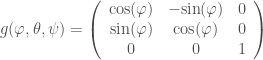
One popular formalism is given by the so-called Euler angles. In this formalism, we break down any arbitrary rotation in -dimensional space into three separate rotations. The first, which we write here by , is expressed as a counterclockwise rotation about the -axis. The second, , is a counterclockwise rotation about an -axis that rotates along with the object. Finally, the third, , is expressed as a counterclockwise rotation about a -axis that, once again, has rotated along with the object. For readers who may be confused, animations of these steps can be found among the references listed at the end of this post.

The matrix which expresses the rotation which is the product of these three rotations can then be written as

.

The reader may check that, in the case that the rotation is strictly in the – plane, i.e. and are zero, we will obtain

.

Note how the upper left part is an element of , expressing a counterclockwise rotation by an angle , as we might expect.

Contrary to the case of , which is an abelian group, the group is not an abelian group. This means that for two elements and of , the product may not always be equal to the product . One can check this explicitly, or simply consider rotating an object along different axes; for example, rotating an object first counterclockwise by 90 degrees along the -axis, and then counterclockwise again by 90 degrees along the -axis, will not end with the same result as performing the same operations in the opposite order.

We now know how to express rotations in -dimensional space using orthogonal matrices. Now we discuss another way of expressing the same concept, but using “unitary”, instead of orthogonal, matrices. However, first we must revisit rotations in dimensions.

The group is not the only way we have of expressing rotations in -dimensions. For example, we can also make use of the unitary (we will explain the meaning of this word shortly) group in -dimension, also written . It is the group formed by the complex numbers with magnitude equal to . The elements of this group can always be written in the form , where is the angle of our rotation. As we have seen in Connection and Curvature in Riemannian Geometry, this group is related to quantum electrodynamics, as it expresses the gauge symmetry of the theory.

The groups and are actually isomorphic. There is a one-to-one correspondence between the elements of and the elements of which respects the group operation. In other words, there is a bijective function , which satisfies for , elements of . When two groups are isomorphic, we may consider them as being essentially the same group. For this reason, both and are often referred to as the circle group.

We can now go back to rotations in dimensions and discuss the group , the special unitary group in dimension . The word “unitary” is in some way analogous to “orthogonal”, but applies to vectors with complex number entries.

Consider an arbitrary vector

.

An orthogonal matrix, as we have discussed above, preserves the quantity (which is the square of what we have referred to earlier as the “magnitude” for vectors with real number entries)

while a unitary matrix preserves

where denotes the complex conjugate of the complex number . This is the square of the analogous notion of “magnitude” for vectors with complex number entries.

Just as orthogonal matrices must satisfy the condition

,

unitary matrices are required to satisfy the condition

where is the Hermitian conjugate of , a matrix whose entries are the complex conjugates of the entries of the transpose of .

An element of the group is therefore a unitary matrix whose determinant is equal to . Like the group , the group is also a group which is not abelian.

Unlike the analogous case in dimensions, the groups and are not isomorphic. There is no one-to-one correspondence between them. However, there is a homomorphism from to that is “two-to-one”, i.e. there are always two elements of that get mapped to the same element of under this homomorphism. Hence, is often referred to as a “double cover” of .

In physics, this concept underlies the weird behavior of quantum-mechanical objects called spinors (such as electrons), which require a rotation of 720, not 360, degrees to return to its original state!

The groups we have so far discussed are not “merely” groups. They also possesses another kind of mathematical structure. They describe certain shapes which happen to have no sharp corners or edges. Technically, such a shape is called a manifold, and it is the object of study of the branch of mathematics called differential geometry, which we have discussed certain basic aspects of in Geometry on Curved Spaces and Connection and Curvature in Riemannian Geometry.

For the circle group, the manifold that it describes is itself a circle. The elements of the circle group correspond to the points of the circle. The group is the surface of the – dimensional sphere, or what we call a -sphere (for those who might be confused by the terminology, recall that we are only considering the surface of the sphere, not the entire volume, and this surface is a -dimensional, not a -dimensional, object). The group is -dimensional real projective space, written . It is a manifold which can be described using the concepts of projective geometry (see Projective Geometry).

A group that is also a manifold is called a Lie group (pronounced like “lee”) in honor of the mathematician Marius Sophus Lie who pioneered much of their study. Lie groups are very interesting objects of study in mathematics because they bring together the techniques of group theory and differential geometry, which teaches us about Lie groups on one hand, and on the other hand also teaches us more about both group theory and differential geometry themselves.

References:

Orthogonal Group on Wikipedia

Rotation Group SO(3) on Wikipedia

Euler Angles on Wikipedia

Unitary Group on Wikipedia

Spinor on Wikipedia

Lie Group on Wikipedia

Real Projective Space on Wikipedia

Algebra by Michael Artin

An Intuitive Introduction to String Theory and (Homological) Mirror Symmetry

String theory is by far the most popular of the current proposals to unify the as of now still incompatible theories of quantum mechanics and general relativity. In this post we will give a short overview of the concepts involved in string theory, but not with the goal of discussing the theory itself in depth (hopefully there will be more posts in the future working towards this task). Instead, we will focus on introducing a very interesting and very beautiful branch of mathematics that arose out of string theory called mirror symmetry. In particular, we will focus on a version of it originally formulated by the mathematician Maxim Kontsevich in 1994 called homological mirror symmetry.

We will start with string theory. String theory started out as a theory of the nuclear forces that held together the protons and electrons in the nucleus of an atom. It was abandoned later on, due to a more successful theory called quantum chromodynamics taking its place. However, it was soon found out that string theory could model the elusive graviton, a particle “carrier” of gravity in the same way that a photon is a particle “carrier” of electromagnetism (the photon is more popularly referred to as a particle of light, but because light itself is an electromagnetic wave, it is also a manifestation of an electromagnetic field), and since then physicists have started developing string theory, no longer in the sole context of nuclear forces, but as a possible candidate for a working theory of quantum gravity.

The incompatibility of quantum mechanics and general relativity (which is currently our accepted theory of gravity) arises from the nonrenormalizability of gravity. In calculations in quantum field theory (see Some Basics of Relativistic Quantum Field Theory and Some Basics of (Quantum) Electrodynamics), there appear certain “nonsensical” quantities which are made sense of via a “corrective” procedure called renormalization (not to be confused with some other procedures called “normalization”). While the way that renormalization works is not really completely understood at the moment, it is known that this procedure at least “works” – this means that it produces the correct values of quantities, as can be checked via experiment.

Renormalization, while it works for the other forces, however fails for gravity. Roughly this is sometimes described as gravity “wildly fluctuating” at the smallest scales. What we know is that this signals, for us, a lack of knowledge of  what physics is like at these extremely small scales (much smaller than the current scale of quantum mechanics).

String theory attempts to solve this conundrum by proposing that particles, at the very smallest scales, are not “particles” at all, but “strings”. This takes care of the problem of fluctuations at the smallest scales, since there is a limit to how small the scale can be, set by the length of the strings. It is perhaps worth noting at this point that the next most popular contender to string theory, loop quantum gravity, tackles this problem by postulating that space itself is not continuous, but “discretized” into units of a certain length. For both theories, this length is predicted to be around meters, a constant quantity which is known as the Planck length.

Over time, as string theory was developed, it became more ambitious, aiming to provide not only the unification of quantum mechanics and general relativity, but also the unification of the four fundamental forces – electromagnetism, the weak nuclear force, the strong nuclear force, and gravity, under one “theory of everything“. At the same time, it needed more ingredients – to be able to account for bosons, the particles carrying “forces”, such as photons and gravitons, and the fermions, particles that make up matter, such as electrons, protons, and neutrons, a new ingredient had to be added, called supersymmetry. In addition, it worked not in the four dimensions of spacetime that we are used to, but instead required ten dimensions (for the “bosonic” string theory, before supersymmetry, the number of dimensions required was a staggering twenty-six)!

How do we explain spacetime having ten dimensions, when we experience only four? It turns out, even before string theory, the idea of extra dimensions was already explored by the physicists Theodor Kaluza and Oskar Klein. They proposed a theory unifying electromagnetism and gravity by postulating an “extra” dimension which was “curled up” into a loop so small we could never notice it. The usual analogy is that of an ant crossing a wire – when the radius of the wire is big, the ant realizes that it can go sideways along the wire, but when the radius of the wire is small, it is as if there is only one dimension that the ant can move along.

So we now have this idea of six curled up dimensions of spacetime, in addition to the usual four. It turns out that there are so many ways that these dimensions can be curled up. This phenomenon is called the string theory landscape, and it is one of the biggest problems facing string theory today. What could be the specific “shape” in which these dimensions are curled up, and why are they not curled up in some other way? Some string theorists answer this by resorting to the controversial idea of a multiverse, so that there are actually several existing universes, each with its own way of how the extra six dimensions are curled up, and we just happen to be in this one because, perhaps, this is the only one where the laws of physics (determined by the way the dimensions are curled up) are able to support life. This kind of reasoning is called the anthropic principle.

In addition to the string theory landscape, there was also the problem of having several different versions of string theory. These problems were perhaps alleviated by the discovery of mysterious dualities. For example, there is the so-called T-duality, where a compactification (a “curling up”) with a bigger radius gives the same laws of physics as a compactification with a smaller, “reciprocal” radius. Not only do the concept of dualities connect the different ways in which the extra dimensions are curled up, they also connect the several different versions of string theory! In 1995, the physicist Edward Witten conjectured that this is perhaps because all these different versions of string theory come from a single “mother theory”, which he called “M-theory“.

In 1991, physicists Philip Candelas, Xenia de la Ossa, Paul Green, and Linda Parkes used these dualities to solve a mathematical problem that had occupied mathematicians for decades, that of counting curves on a certain manifold (a manifold is a shape without sharp corners or edges) known as a Calabi-Yau manifold. In the context of Calabi-Yau manifolds, which are some of the shapes in which the extra dimensions of spacetime are postulated to be curled up, these dualities are known as mirror symmetry. With the success of Candelas, de la Ossa, Green, and Parkes, mathematicians would take notice of mirror symmetry and begin to study it as a subject of its own.

Calabi-Yau manifolds are but special cases of Kahler manifolds, which themselves are very interesting mathematical objects because they can be studied using three aspects of differential geometry – Riemannian geometry, symplectic geometry, and complex geometry.

We have already encountered examples of Kahler manifolds on this blog – they are the elliptic curves (see Elliptic Curves and The Moduli Space of Elliptic Curves). In fact elliptic curves are not only Kahler manifolds but also Calabi-Yau manifolds, and they are the only two-dimensional Calabi-Yau manifolds (we sometimes refer to them as “one-dimensional” when we are considering “complex dimensions”, as is common practice in algebraic geometry – this apparent “discrepancy” in counting dimensions arises because we need two real numbers to specify a complex number). In string theory of course we consider six-dimensional (three-dimensional when considering complex dimensions) Calabi-Yau manifolds, since there are six extra curled up dimensions of spacetime, but often it is also fruitful to study also the other cases, especially the simpler ones, since they can serve as our guide for the study of the more complicated cases.

Riemannian geometry studies Riemannian manifolds, which are manifolds equipped with a metric tensor, which intuitively corresponds to an “infinitesimal distance formula” dependent on where we are on the manifold. We have already encountered Riemannian geometry before in Geometry on Curved Spaces and Connection and Curvature in Riemannian Geometry. There we have seen that Riemannian geometry is very important in the mathematical formulation of general relativity, since in this theory gravity is just the curvature of spacetime, and the metric tensor expresses this curvature by showing how the formula for the infinitesimal distance between two points (actually the infinitesimal spacetime interval between two events) changes as we move around the manifold.

Symplectic geometry, meanwhile, studies symplectic manifolds. If Riemannian manifolds are equipped with a metric tensor that measures “distances”, symplectic manifolds are equipped with a symplectic form that measures “areas”. The origins of symplectic geometry are actually related to William Rowan Hamilton’s formulation of classical mechanics (see Lagrangians and Hamiltonians), as developed later on by Henri Poincare. There the object of study is phase space, which gives the state of a system based on the position and momentum of the objects that comprise it. It is this phase space that is expressed as a symplectic manifold.

Complex geometry, following our pattern, studies complex manifolds. These are manifolds which locally look like , in the same way that ordinary differentiable manifolds locally look like . Just as Riemannian geometry has metric tensors and symplectic geometry has symplectic forms, complex geometry has complex structures, mappings of tangent spaces with the property that applying them twice is the same as multiplication by , mimicking the usual multiplication by the imaginary unit on the complex plane.

Complex manifolds are not only part of differential geometry, they are also often studied using the methods of algebraic geometry! We recall (see Basics of Algebraic Geometry) that algebraic geometry studies varieties and schemes, which are shapes such as lines, conic sections (parabolas, hyperbolas, ellipses, and circles), and elliptic curves, that can be described by polynomials (their modern definitions are generalizations of this concept). In fact, all Calabi-Yau manifolds can be described by polynomials, such as the following example, due to user Andrew J. Hanson of Wikipedia:

This is a visualization (actually a sort of “cross section”, since we can only display two dimensions and this object is actually six-dimensional) of the Calabi-Yau manifold described by the following polynomial equation:

This polynomial equation (known as the Fermat quintic) actually describes the Calabi-Yau manifold  in projective space using homogeneous coordinates. This means that we are using the concepts of projective geometry (see Projective Geometry) to include “points at infinity“.

We note at this point that Kahler manifolds and Calabi-Yau manifolds are interesting in their own right, even outside of the context of string theory. For instance, we have briefly mentioned in Algebraic Cycles and Intersection Theory the Hodge conjecture, one of seven “Millenium Problems” for which the Clay Mathematics Institute is currently offering a million-dollar prize, and it concerns Kahler manifolds. Perhaps most importantly, it “unifies” several different branches of mathematics; as we have already seen, the study of Kahler manifolds and Calabi-Yau manifolds involves Riemannian geometry, symplectic geometry, complex geometry, and algebraic geometry. The more recent version of mirror symmetry called homological mirror symmetry further adds category theory and homological algebra to the mix.

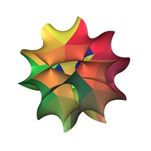
Now what mirror symmetry more specifically states is that a version of string theory called Type IIA string theory, on a spacetime with extra dimensions compactified onto a certain Calabi-Yau manifold , is the same as another version of string theory, called Type IIB string theory, on a spacetime with extra dimensions compactified onto another Calabi-Yau manifold , which is “mirror” to the Calabi-Yau manifold .

The statement of homological mirror symmetry (which is still conjectural, but mathematically proven in certain special cases) expresses the idea of the previous paragraph as follows (quoted verbatim from the paper Homological Algebra of Mirror Symmetry by Maxim Kontsevich):

Let be a -dimensional symplectic manifold with and be a dual -dimensional complex algebraic manifold.

The derived category constructed from the Fukaya category (or a suitably enlarged one) is equivalent to the derived category of coherent sheaves on a complex algebraic variety .

The statement makes use of the language of category theory and homological algebra (see Category Theory, More Category Theory: The Grothendieck Topos, Even More Category Theory: The Elementary Topos, Exact Sequences, More on Chain Complexes, and The Hom and Tensor Functors), but the idea that it basically expresses is that there exists a relation between the symplectic aspects of the Calabi-Yau manifold , as encoded in its Fukaya category, and the complex aspects of the Calabi-Yau manifold , as encoded in its category of coherent sheaves (see Sheaves and More on Sheaves). As we have said earlier, the subjects of algebraic geometry and complex geometry are closely related, and hence the language of sheaves show up in (and is an important part of) both subjects. The concept of derived categories, which generalize derived functors like the Ext and Tor functors, allow us to relate the two categories, which otherwise would be expressing different concepts. Inspired by string theory, therefore, we have now a deep and beautiful idea in geometry, relating its different aspects.

Is string theory the correct way towards a complete theory of quantum gravity, or the so-called “theory of everything”? As of the moment, we don’t know. Quantum gravity is a very difficult problem, and the scales involved are still far out of our reach – in order to probe smaller and smaller scales we need particle accelerators with higher and higher energies, and right now the technologies that we have are still very, very far from the scales which are relevant to quantum gravity. Still, it is hoped for that whatever we find in experiments in the near future, not only in the particle accelerators but also in the radio telescopes that look out into space, will at least guide us towards the correct path.

There are some who believe that, in the absence of definitive experimental evidence, mathematical beauty is our next best guide. And, without a doubt, string theory is related to, and has inspired, some very beautiful and very interesting mathematics, including that which we have discussed in this post. Still, physics, like all natural science, is empirical (based on evidence and observation), and hence it is ultimately physical evidence that will be the judge of correctness. It may yet turn out that string theory is wrong, and that it is a different theory which describes the fundamental physical laws of nature, or that it needs drastic modifications to its ideas. This will not invalidate the mathematics that we have described here, anymore than the discoveries of Copernicus invalidated the mathematics behind the astronomical model of Ptolemy – in fact this mathematics not only outlived the astronomy of Ptolemy, but served the theories of Copernicus, and his successors, just as well. Hence we cannot really say that the efforts of Ptolemy were wasted, since even though his scientific ideas were shown to be wrong, still his mathematical methods were found very useful by those who succeeded him. Thus, while our current technological limitations prohibit us from confirming or ruling out proposals for a theory of quantum gravity such as string theory, there is still much to be gained from such continued efforts on the part of theory, while experiment is still in the process of catching up.

Our search for truth continues. Meanwhile, we have beauty to cultivate.

References:

String Theory on Wikipedia

Mirror Symmetry on Wikipedia

Homological Mirror Symmetry on Wikipedia

Calabi-Yau Manifold on Wikipedia

Kahler Manifold on Wikipedia

Riemannian Geometry on Wikipedia

Symplectic Geometry on Wikipedia

Complex Geometry on Wikipedia

Fukaya Category on Wikipedia

Coherent Sheaf on Wikipedia

Derived Category on Wikipedia

Image by User Andrew J. Hanson of Wikipedia

Homological Algebra of Mirror Symmetry by Maxim Kontsevich

The Elegant Universe: Superstrings, Hidden Dimensions, and the Quest for the Ultimate Theory by Brian Greene

String Theory by Joseph Polchinski

String Theory and M-Theory: A Modern Introduction by Katrin Becker, Melanie Becker, and John Schwarz

Some Basics of Statistical Mechanics

The branch of physics now known as statistical mechanics started out as thermodynamics, the study of heat and related concepts. The relation of thermodynamics to the rest of physics, i.e. the relation of heat and motion, was studied by scientists like James Prescott Joule in the 19th century. Due to their efforts, we have the idea that what they used to refer to as “heat” is a form of energy which is transferred from one object to another, manifesting in ways other than the bulk motion of the objects (in particular, as a change in the “internal energy” of the objects involved) .

Energy, a concept that was already associated to the motion of objects (see also Lagrangians and Hamiltonians), can be transferred from one object to another, or one system to another, and in the case of heat, this transfer involves the concept of temperature. Temperature is what we measure on a thermometer, and when we say something is “hot” or “cold”, we are usually referring to its temperature.

The way by which temperature dictates the direction in which heat is transferred is summarized in the second law of thermodynamics (here we give one of its many equivalent statements):

Heat flows from a hotter object to a colder one.

This process of transfer of heat will continue, decreasing the internal energy of the hotter object and increasing the internal energy of the cooler one, until the two objects have equal temperatures, in which case we say that they are in thermal equilibrium.

But if heat is a transfer of energy, and energy is associated to motion, then what was it, exactly, that was moving (or had the capacity to cause something to move)? What is this “internal energy?” For us, who have been taught about atoms and molecules since childhood, the answer might come rather easily. Internal energy is the energy that comes from the motion of the atoms and molecules that comprise the object. But for the scientists who were developing the subject during the 19th century, the concept of atoms and molecules was still in its very early stages, with many of them facing severe criticism for adopting ideas that at the time were still not completely verified.

Still, these scientists continued to take the point of view that the subject of thermodynamics was just the same physics that had already been applied to, say, the motion of cannonballs and pendulums and other objects, except that now they had to be applied to a very large quantity of very small particles (quantum mechanics would later have much to contribute also, but even before the introduction of that theory the concept of atoms and molecules was already starting to become very fruitful in thermodynamics).

Now we have an explanation for what internal energy is in terms of the motion of the particles that make up an object. But what about temperature? It is possible to explain temperature (and therefore the laws that decide the direction of the transfer of heat) using more “basic” concepts such as Newton’s laws of motion, like we have done for the internal energy?

It was the revolutionary ideas of Ludwig Boltzmann that provided the solution. It indeed involved a more “basic” concept, but not one we would usually think of as belonging to the realm of physics or the study of motion. The idea of Boltzmann was to relate temperature to the concepts of information, probability, and statistics, via the notion of entropy. We may therefore think of this era as the time when “thermodynamics” became “statistical mechanics”.

In order to discuss the idea of entropy, for a moment we step away from physics, and discuss instead cards. It is not cards themselves that we are interested in, but information. Entropy is really about information, which is why it also shows up, for instance, when discussing computer passwords. Cards will give us a simple but concrete way to discuss information.

Consider now, therefore, a deck of 52 ordinary playing cards. A hand, of course, consists of five cards. Using the rules of combinatorics, we can find that there are 2,598,960 different hands (combinations of 52 different playing cards taken five at a time, in any order). In the game of poker, there are certain special combinations, the rarest (and highest-ranking) of which is called the “royal flush”. There are only four possible ways to get a royal flush (one for each suit). In contrast, the most common kind of hand is one which has no special combination (sometimes called “no pair”), and there are 1,302,540 different combinations which fit this description.

Now suppose the deck is shuffled and we are dealt a hand. The shuffling process is not entirely random (not in the way that quantum mechanics is), but there are so many things going on that it is near-impossible for us to follow and determine what kind of hand we are going to get. The most we can do is make use of what we know about probability and statistics. We know that it is more likely for us to obtain a no pair rather than a royal flush, simply because there are so many more combinations that are considered a no pair than there are combinations that are considered a royal flush. There are no laws of physics involved in making this prediction; there is only the intuitive idea that an event with more ways of happening is more likely to happen compared to an event with less ways of happening, in the absence of any more information regarding the system.

We now go back to physics. Let us consider a system made up of a very large number of particles. The state of a single particle is specified by its position and momentum, and the state of the entire system is specified by the position and momentum of every one of its particles. This state is almost impossible for us to determine, because there are simply too many particles to keep track of.

However, we may be able to determine properties of the system without having to look at every single particle. Such properties may involve the total energy, pressure, volume, and so on. These properties determine the “macrostate” of a system. The “true” state that may only be specified by the position and momentum of every single particle is called the “microstate” of the system. There may be several different microstates that correspond to a single macrostate, just like there are four different combinations that correspond to a royal flush, or 1,302,540 different combinations that correspond to a no pair.

Let the system be in a certain macrostate, and let the number of microstates that correspond to this macrostate be denoted by . The entropy of the system is then defined as

.

where is a constant known as Boltzmann’s constant. We may think of this constant and the logarithm as merely convenient ways (in terms of calculation, and in terms of making contact with older ideas in thermodynamics) to express the idea that the higher the number of microstates, the higher the entropy.

Now even though the system may not seem to be changing, imperceptible to us, there may be many things that happen on a microscopic level. Molecules may be moving around in many directions, in motions that are too difficult for us to keep track of, not only because the particles are very small but also because there are just too many of them. This is analogous to the shuffling of cards. All that we have at our disposal are the tools of probability and statistics. Hence the term, “statistical mechanics“.

What have we learned from the example of the shuffling of cards? Even though we could not keep track of things and determine results, we could still make predictions. And the predictions we made were simply of the nature that an event with more ways of happening was more likely to happen than an even with less ways of happening.

Therefore, we have the following restatement of the second law of thermodynamics:

The entropy of a closed system never decreases.

This simply reflects the idea that under these processes we cannot keep track of, the system is more likely to adopt a configuration with more ways of happening, compared to one with less ways of happening. In other words,it will be in a macrostate that will have more microstates. Microscopically, it may happen that “miraculously” the entropy increases; but given how many particles there are, and how many processes happen, this is extremely unlikely to be a sustained phenomenon, and macroscopically, the second law of thermodynamics is always satisfied. This is like obtaining a royal flush on one deal of cards; but if we are going to reshuffle multiple times, it is unlikely that we keep getting royal flushes for a sustained period of time.

The “closed system” requirement is there to ensure that the system is “left to its own devices” so to speak, or that there is no “outside interference”.

Considering that the entirety of the universe is an example of a “closed system” (there is nothing outside of it, since by definition the universe means the collection of everything that exists), the second law of thermodynamics has some interesting (perhaps disturbing, to some people) implications. What we usually consider to be an “ordered” configuration is very specific; for example, a room is only in order when all of the furniture is upright, all the trash is in the wastebasket, and so on. There are fewer such configurations compared to the “disordered” ones, since there are so many ways in which the furniture can be “not upright”, and so many ways in which the trash may be outside of the wastebasket, etc. In other words, disordered configurations have higher entropy. All of these things considered, what the second law of thermodynamics implies is that the entropy of the universe is ever increasing, moving toward an increasing state of disorder, away from the delicate state of order that we now enjoy.

We now want to derive the “macroscopic” from the “microscopic”. We want to connect the “microscopic” concept of entropy to the “macroscopic” concept of temperature. We do this by defining “temperature” as the following relationship between the entropy and the energy (in this case the internal energy, as the system may have other kinds of energy, for example arising from its motion in bulk):

Although we will not discuss the specifics in this post, we make the following claim – the entropy of the system is at its maximum when the system is in thermal equilibrium. Or perhaps more properly, the state of “thermal equilibrium” may be defined as the macrostate which has the most amount of microstates corresponding to it. This in turn explains why heat flows from a hotter object to a cooler one.

We have now discussed some of the most basic concepts in thermodynamics and statistical mechanics. We now briefly discuss certain technical and calculational aspects of the theory. Aside from making the theory more concrete, this is important also because there are many analogies to be made outside of thermodynamics and statistical mechanics. For example, in the Feynman path integral formulation of quantum field theory (see Some Basics of Relativistic Quantum Field Theory) we calculate correlation functions, which mathematically have a form very similar to some of the quantities that we will discuss.

In modern formulations of statistical mechanics, a central role is played by the partition function , which is defined as

where , often simply referred to as the “thermodynamic beta”, is defined as

.

The partition function is a very convenient way to package information about the system we are studying, and many quantities of interest can be obtained from it. One of the most important ones is the probability for the system to be in a macrostate with energy :

.

Knowing this formula for the probabilities of certain macrostates allows us to derive the formulas for expectation values of quantities that may be of interest to us, such as the average energy of the system:

.

After some manipulation we may find that the expectation value of the energy is also equal to the following more compact expression:

.

Another familiar quantity that we can obtain from the partition function is the entropy of the system:

.

There are various other quantities that can be obtained from the partition function, such as the variance of the energy (or energy fluctuations), the heat capacity, and the so-called Helmholtz free energy. We note that for “continuous” systems, expressions involving sums are replaced by expressions involving integrals. Also, for quantum mechanical systems, there are some modifications, as well as for systems which exchange particles with the environment.

The development of statistical mechanics, and the introduction of the concept of entropy, is perhaps a rather understated revolution in physics. Before Boltzmann’s redefinition of these concepts, physics was thought of as studying only motion, in the classical sense of Newton and his contemporaries. Information has since then taken just as central a role in modern physics as motion.

The mathematician and engineer Claude Elwood Shannon further modernized the notion of entropy by applying it to systems we would not have ordinarily thought of as part of physics, for example the bits on a computer. According to some accounts, Shannon was studying a certain quantity he wanted to name “information”; however, the physicist and mathematician John von Neumann told him that a version of his concept had already been developed before in physics, and was called “entropy”. With Neumann’s encouragement, Shannon adopted the name, symbolically unifying subjects formerly thought of as separate.

Information theory, the subject which Shannon founded, has together with quantum mechanics led to quantum information theory, which not only has many potential applications in technology but also is one of the methods by which we attempt to figure out deep questions regarding the universe.

Another way in which the concept of entropy is involved in modern issues in physics is in the concept of entropic gravity, where gravity, as expressed in Einstein’s general theory of relativity, is derived from more fundamental concepts similar to how the simple statistical concept of entropy gives rise to something that manifests macroscopically as a law of physics. Another part of modern physics where information, quantum mechanics, and general relativity meet is the open problem called the black hole information paradox, which concerns the way in which black holes seemingly do not conserve information, and is a point of contention among many physicists even today.

Finally, we mention another very interesting aspect of statistical mechanics, perhaps, on the surface, a little more mundane compared to what we have mentioned on the preceding paragraphs, but not the slightest bit less interesting – phase transitions. Phase transitions are “abrupt” changes in the property of an object brought about by some seemingly continuous process, like, for example, the freezing of water into ice. We “cool” water, taking away heat from it by some process, and for a long time it seems that nothing happens except that the water becomes colder and colder, but at some point it freezes – an abrupt change, even though we have done just the same thing we did to it before. What really happens, microscopically, is that the molecules have arranged themselves into a some sort of structure, and the material loses some of symmetry (the “disordered” molecules of water were more symmetric than the “ordered” molecules in ice) – a process known as symmetry breaking. Phase transitions and symmetry breaking are ubiquitous in the sciences, and have applications from studying magnets to tackling the problem of why we have observed so much more matter compared to antimatter.

References:

Thermodynamics on Wikipedia

Statistical Mechanics on Wikipedia

Entropy on Wikipedia

Partition Function on Wikipedia

Entropy in Thermodynamics and Information Theory on Wikipedia

Quantum Information on Wikipedia

Black Hole Information Paradox on Wikipedia

Phase Transition on Wikipedia

Symmetry Breaking on Wikipedia

It From Bit – Entropic Gravity for Pedestrians on Science 2.0

Black Hole Information Paradox: An Introduction on Of Particular Significance

Thermal Physics by Charles Kittel and Herbert Kroemer

Fundamentals of Statistical and Thermal Physics by Frederick Reif

A Modern Course in Statistical Physics by Linda Reichl

Book List

There’s a new page on the blog: Book List. It’s far from comprehensive, but I hope to be able to update it from time to time. I don’t intend to put every book on mathematics and physics on the list of course, just the ones I have read and liked, or heavily recommended by other people. I hope to strike a balance between being somewhat comprehensive, with more than one book on the same subject if they happen to complement each other, and yet not listing too many so as not to confuse people with an overwhelming list of multiple books on the same subjects. Links to older, and more comprehensive, book lists (with helpful reviews) are included at the bottom of the page.