Hilbert Modular Surfaces

June 8, 2023February 14, 2024 / Anton Hilado / Leave a comment

Hilbert Modular Surfaces and Hilbert Modular Forms: The Basics

A Hilbert modular surface is a kind of Shimura variety (see Shimura Varieties), in a sense one of the next simplest after modular curves (although Shimura curves have lower dimension and Siegel modular threefolds have a simpler moduli interpretation). Aside from being a higher-dimensional analogue of modular curves, Hilbert modular surfaces possess interesting structure not present in modular curves. For example, Hilbert modular forms may contain embedded modular curves as codimension $1$ subvarieties!

We begin with the definition. Let $F=\mathbb{Q}(\sqrt{d})$ , where $d$ is a squarefree positive integer, i.e. $F$ is a real quadratic field. We denote its ring of integers by $\mathcal{O}_{F}$ . The group $\Gamma=\mathrm{SL}_{2}(\mathcal{O}_{F})$ acts on the product $\mathbb{H}\times \mathbb{H}$ of two upper half-planes as follows:

$\displaystyle \begin{pmatrix} a & b \\ c & d \end{pmatrix}(z_{1},z_{2})=\left(\frac{az_{1}+b}{cz_{1}+d},\frac{a'z_{2}+b'}{c'z_{2}+d'}\right)$

for $(z_{1},z_{2})\in \mathbb{H}\times\mathbb{H}$ , where $a',b',c',d'$ are the Galois conjugates of $a,b,c,d$ . If we then take the left quotient of $\mathbb{H}\times\mathbb{H}$ by this action of $\Gamma)$ , we then end up with a complex analytic surface $Y(\Gamma)$ , which is non-compact. Just as the “open” modular curve constructed in The Moduli Space of Elliptic Curves parametrizes elliptic curves over $\mathbb{C}$ , the open modular surface $Y(\Gamma)$ which we have just constructed parametrizes abelian surfaces $A$ over $\mathbb{C}$ with an extra “real multiplication” structure, which is an embedding of $\mathcal{O}_{F}$ into their ring of endomorphisms $\mathrm{End}(A)$ .

We may “compactify” the above construction by instead considering the quotient $\Gamma\backslash(\mathbb{H}\times\mathbb{H}\cup\mathbb{P}^1(F))$ (note that $\mathbb{P}^{1}(F)$ is also equipped with an action of $\Gamma$ ), which adds a finite number (equal to the class number of $F$ ) of points called cusps. This compactification, which we denote $X(\Gamma)$ , will be singular. However, by the theory developed by Heisuke Hironaka, there is a way to “resolve” the singularities, and by applying this theory we may obtain a smooth projective surface $\widetilde{X}(\Gamma)$ .

Hilbert modular surfaces are the natural home of Hilbert modular forms (although Hilbert modular forms live on Hilbert modular varieties, more generally, as we mention in the next paragraph). A Hilbert modular form of weight $(k_{1},k_{2})$ is a meromorphic function $f$ on $\mathbb{H}\times\mathbb{H}$ such that, for $\gamma=\begin{pmatrix}a & b \\ c & d\end{pmatrix}\in\Gamma$ , we have

$\displaystyle f(\gamma z)=(cz_{1}+d)^{k_{1}}(c'z_{2}+d')^{k_{2}}f(z_{1},z_{2})$

From the point of view of algebraic geometry, Hilbert modular forms can also be obtained as sections of certain sheaves on a Hilbert modular surface.

Before we continue our discussion of Hilbert modular surfaces, we note that all of the above constructions may be generalized by letting $F$ be a more general totally real field, instead of just a real quadratic field. This leads to the more general notion of a Hilbert modular variety, and of more general Hilbert modular forms. We also note that instead of $\Gamma=\mathrm{SL}_{2}(\mathcal{O}_{F})$ , we could instead consider some nontrivial level structure $\Gamma=\Gamma(\mathcal{O}_{F}\oplus\mathfrak{a})$ , where $\mathfrak{a}$ is some fractional ideal of $\mathcal{O}_{F}$ . The group $\Gamma(\mathcal{O}_{F}\oplus\mathfrak{a})$ is defined to be the group of matrices of the form $\begin{pmatrix} a & b \\ c & d \end{pmatrix}$ where $a,d\in\mathcal{O}_{F}$ , $b\in\mathfrak{a}^{-1}$ , and $c\in\mathfrak{a}$ .

A Whirlwind Introduction to Clifford Algebras and Spin Groups

We have so far described Hilbert modular surfaces and Hilbert modular forms in terms of the group $\mathrm{SL}_{2}(F)$ . However there is another way to describe them via the exceptional isomorphisms of spin groups (which are double covers of special orthogonal groups, see also Rotations in Three Dimensions) with other groups – In our case, we have the isomorphism $\mathrm{Spin}(2,2)\simeq\mathrm{SL}_{2}(F)$ . Let us discuss first the general theory behind spin groups of signature $(2,n)$ and their associated symmetric spaces, and then later we apply it to the specific case of Hilbert modular surfaces.

Let $(V,q)$ be a pair consisting of a vector space $V$ over $\mathbb{Q}$ and a quadratic form $q$ . The orthogonal group $\mathrm{O}(V)$ is the subgroup of the group of linear transformations of $V$ which preserve $q$ . The Clifford algebra $C_{V}$ associated to $(V,q)$ is the quotient of the tensor algebra of $V$ by the relation, for all $v\in V$ ,

$\displaystyle v^{2}=q(v)$

The Clifford algebra generalizes many familiar constructions such as the complex numbers (for $V=\mathbb{R}$ and $q(v)=-v^{2}$ ) and Hamilton’s quaternions for $V=\mathbb{R}^{2}$ and $q(v_{1}+v_{2})=-v_{1}^{2}-v_{2}^{2}$ . Note that, unlike the complex numbers, more general Clifford algebras such as Hamilton’s quaternions have more than one type of “conjugation”. The first, which we shall call $J$ , is induced by negation of basis elements of $V$ . Another is given by cyclically permuting the tensor factors of an element so that $x^{t}=v_{2}\otimes\ldots \otimes v_{m}\otimes v_{1}$ for $v=v_{1}\otimes\ldots\otimes v_{m}$ . This second conjugation allows us to define the Clifford norm:

$\displaystyle \mathrm{Nm}(v)=v^{t}v$

The even Clifford algebra $C_{V}^{0}$ of $C_{V}$ is the subalgebra generated by elements which are a product of an even number of basis elements of $V$ . The odd part $C_{V}^{1}$ is similarly defined, and we have the decomposition $C_{V}=C_{V}^{0}\oplus C_{V}^{1}$ . The Clifford group is defined to be the set of all invertible elements $v$ of the Clifford algebra such that $vVJ(v)^{-1}=V$ . The intersection of the even Clifford algebra and the Clifford group is called $\mathrm{GSpin}(V)$ . The set of elements of $\mathrm{GSpin}(V)$ whose Clifford norm is equal to $1$ is called $\mathrm{Spin}(V)$ .

We now mention some facts about the special case when $V$ has dimension $4$ that we will use later when we discuss Hilbert modular surfaces again. Let $v_{1},v_{2},v_{3},v_{4}$ be a basis of $V$ such that $q(v_{i})\neq 0$ for all $i$ . Let $\delta=v_{1}v_{2}v_{3}v_{4}$ . The center $Z$ of the Clifford algebra associated to $(V,q)$ is then isomorphic to $\mathbb{Q}+\mathbb{Q}\delta$ , and the even Clifford algebra admits the description

$\displaystyle C_{V}^{0}=Z+Zv_{1}v_{2}+Zv_{2}v_{3}+Zv_{1}v_{3}$

Fix an element $v_{0}\in V$ such that $q(v_{0})\neq 0$ and for $v\in C_{V}^{0}$ let $v^{\sigma}=v_{0}vv_{0}^{-1}$ . We define the new vector space $\widetilde{V}$ to be the set of all elements $v$ of $C_{V}^{0}$ such that the automorphism $v^{\sigma}$ agrees with the conjugation $v^{t}$ , and we equip $\widetilde{V}$ with the quadratic form $\widetilde{q}(v)=q(v_{0})\cdot \mathrm{Nm}(v)$ . It turns out that $(\widetilde{V},\widetilde{q})$ is isometric to $(V,q)$ , and the upshot is that we can now describe the action of an element $g\in\mathrm{Spin}(V)$ on an element $v\in\widetilde{V}$ as follows:

$\displaystyle g(v)=gVg^{-\sigma}$ .

Symmetric Spaces for Orthogonal Groups of Signature (2,n): Three Descriptions

The upper-half plane is the “symmetric space” for the group $\mathrm{SL}_{2}(\mathbb{R})$ , and may be obtained as the quotient of $\mathrm{SL}_{2}(\mathbb{R})$ by its locally compact subgroup $\mathrm{SO}(2)$ . We want to generalize this to the group $\mathrm{O}(V)$ , but it is often useful to have different descriptions of the symmetric space. We will discuss three different descriptions of the symmetric space on which $\mathrm{O}(V)$ acts, each one with its own advantages and disadvantages.

First we give the “Grassmannian model“. The Grassmannian parametrizes $k$ -dimensional subspaces of a vector space. It is a generalization of projective space (which is the special case when $k=1$ ). In our case, we want to parametrize $2$ -dimensional spaces of $V$ , with the additional condition that the quadratic form $q$ is positive definite on this space:

$\displaystyle \mathrm{Gr}(V)=\lbrace v\in V:\mathrm{dim}(v)=2\mbox{ and }q\vert_{v}>0\rbrace$

The group $\mathrm{O}(V)$ acts on $\mathrm{Gr}(V)$ , and the stabilizer of an element $v_{0}$ is a maximal compact subgroup $K$ , which is isomorphic to $\mathrm{O}(2)\times \mathrm{O}(n)$ . Therefore we can see that $\mathrm{Gr}(V)\cong \mathrm{O}(V)/K$ , and provides a realization of its associated symmetric space. However, in this model it is harder to see the complex analytic structure.

This problem can be remedied by considering the “projective model“. Let $V(\mathbb{C})$ be the complexification of $V$ and define

$\displaystyle \mathcal{K}=\lbrace[z]\in\mathbb{P}(V(\mathbb{C})):(z,z)=0,(z,\overline{z})>0\rbrace$

Now $\mathcal{K}$ is an $n$ -dimensional complex manifold consisting of two connected components. We choose one of these components and denote it by $\mathcal{K}^{+}$ – this is our symmetric space. Although the complex analytic structure is easier to see in the projective model, it is hard to relate this model to well-known examples of symmetric spaces such as the upper half-plane (which is the case when $n=1$ ).

Finally we consider the “tube domain model“. Let $e_{1}$ be a nonzero isotropic vector in $V$ and let $e_{2}$ be another vector in $V$ such that $(e_{1},e_{2})=1$ . We let $W$ be the intersection of the orthogonal complements of $e_{1}$ and $e_{2}$ in $V$ , so that

$\displaystyle V=W\oplus \mathbb{C}e_{1}\oplus\mathbb{C}e_{2}$

On the vector space $W$ , the restriction of the quadratic form $q$ has signature $1,n-1$ . We let $W(\mathbb{C})$ denote the complexification of $W$ and define

$\displaystyle \mathcal{H}=\lbrace z\in W(\mathbb{C}):q(\mathrm{Im}(z))>0)\rbrace$

We can define a biholomorphic map between $\mathcal{H}$ and $\mathcal{K}$ by sending $z$ to $[(z,1,-q(z)-q(e_{2}))]$ . We denote the preimage of $\mathcal{K}^{+}$ by $\mathcal{H}^{+}$ – the latter is analogous to the upper half-plane.

Heegner Divisors

Let us now consider smaller modular varieties embedded in other bigger modular varieties. Let $L$ be a lattice in $V$ . The idea is that if we pick a vector $\lambda$ in the dual lattice $L^{\vee}$ in $V$ , and consider the orthogonal complement of $\lambda$ in $V$ , what we get is actually a vector space of signature $2,n-1$ , to which we can once again apply the preceding constructions! Applied to the case of Hilbert modular surfaces, this explains the embedded modular curves. In symbols, we have

$\displaystyle H_{\lambda}=\lbrace [Z]\in\mathcal{K}^{+}:(Z,\lambda)=0\rbrace$

If we write $\lambda=\lambda_{W}+ae_{2}+be_{1}$ , then we can also describe $H_{\lambda}$ in the tube domain model as follows:

$\displaystyle H_{\lambda}=\lbrace z\in\mathcal{H}^{+}:aq(z)-(z,\lambda_{W})-aq(e_{2})-b=0\rbrace$

We can now define the Heegner divisor $H(\beta,m)$ as the sum of all the $H_{\lambda}$ where $\lambda\in\beta+L$ satisfies the condition that $q(\lambda)=m$ . We can further define the composite Heegner divisor $H(m)$ as half the sum of all Heegner divisors $H(\beta,m)$ as $\beta$ runs over $L^{\vee}/L$ .

Back to Hilbert Modular Surfaces

We now go back to our setting of Hilbert modular surfaces and apply the above theory to the $4$ -dimensional vector space $V=\mathbb{Q}\oplus\mathbb{Q}\oplus F$ , equipped with the quadratic form $q(a,b,\nu)=\nu\nu'-ab$ . We choose the following basis for $V$ :

$\displaystyle v_{1}=(1,1,0)$

$\displaystyle v_{2}=(1,-1,0)$

$\displaystyle v_{3}=(0,0,1)$

$\displaystyle v_{4}=(0,0,\sqrt{d})$

In this case the center of the Clifford algebra is isomorphic to $F$ , and the even Clifford algebra $C_{V}^{0}$ of $V$ is of the form $C_{V}^{0}=F+Fv_{1}v_{2}+Fv_{2}v_{3}+Fv_{1}v_{3}$ . Via the assignments

$\displaystyle 1\mapsto\begin{pmatrix}1 & 0 \\ 0 & 1\end{pmatrix}$

$\displaystyle v_{1}v_{2}\mapsto\begin{pmatrix}1 & 0 \\ 0 & -1\end{pmatrix}$

$\displaystyle v_{2}v_{3}\mapsto\begin{pmatrix}0 & 1 \\ -1 & 0\end{pmatrix}$

$\displaystyle v_{1}v_{3}\mapsto\begin{pmatrix}0 & 1 \\ 1 & 0\end{pmatrix}$

we have an isomorphism between $C_{V}^{0}$ and $M_{2}(F)$ . Furthermore, the Clifford norm on $C_{V}^{0}$ corresponds to the determinant on $M_{2}(F)$ . All in all, this gives us an isomorphism between $\mathrm{Spin}_{V}$ and $\mathrm{SL}_{2}(F)$ . The theory we have discussed earlier provides us with the following vector space $\widetilde{V}$ isomorphic to $V$ :

$\displaystyle \widetilde{V}=\left\lbrace \begin{pmatrix} a & \nu' \\ \nu & b\end{pmatrix}:a,b\in\mathbb{Q},\nu\in F\right\rbrace$

We also have a description of the lattices $L$ and $L^{\vee}$ as matrices inside $\widetilde{V}$ as follows:

$\displaystyle L=\mathbb{Z}\oplus\mathbb{Z}\oplus\mathcal{O}_{F}=\left\lbrace\begin{pmatrix}a & \nu' \\ \nu' & b\end{pmatrix}:a,b\in\mathbb{Z},\nu\in\mathcal{O}_{F}\right\rbrace$

$\displaystyle L^{\vee}=\mathbb{Z}\oplus\mathbb{Z}\oplus\mathfrak{d}^{-1}=\left\lbrace\begin{pmatrix}a & \nu' \\ \nu' & b\end{pmatrix}:a,b\in\mathbb{Z},\nu\in\mathcal{O}_{F}\right\rbrace$

It turns out, just as we have $\mathrm{Spin}(V)\cong \mathrm{SL}_{2}(F)$ , we also have $\mathrm{Spin}(L)\cong\mathrm{SL}_{2}(\mathcal{O}_{F})$ . In turn this gives us an isomorphism $Y(\Gamma)\cong Y(\mathrm{Spin}(L))$ .

Now we apply the general theory of Heegner divisors. In the special case of Hilbert modular surfaces, the Heegner divisors $H(-m/D)$ where $D$ is the discriminant of $F$ are also known as Hirzebruch-Zagier divisors. They have the explicit description

$\displaystyle T_{m}=\sum\lbrace(z_{1},z_{2}\in\mathbb{H}\times\mathbb{H}):az_{1}z_{2}+\lambda z_{1}+\lambda' z_{2}+b\rbrace$

where the sum is over all $(a,b,\lambda)\in L^{\vee}/\lbrace\pm 1\rbrace$ such that $ab-\lambda\lambda'=m$ . As a special case, $T_{1}$ is the modular curve of level $1$ (i.e. the compactified moduli space of elliptic curves).

Borcherds Products and the Kudla Program: A Preview

Hirzebruch-Zagier divisors are related to certain Hilbert modular forms called Borcherds products, which arise as “theta lifts” (see also The Theta Correspondence) of weakly holomorphic modular forms (which are almost the same as modular forms, but the holomorphicity condition at the cusps is relaxed). Here “theta lifts” is in quotes because the liftings are somewhat different from what is described in The Theta Correspondence; for one, the integral is divergent and requires a “regularization” to get it to converge, and the lifting is multiplicative, which gives it an expression as an infinite product – hence the name “Borcherds products”.

The Hirzebruch-Zagier divisors, or more generally the Heegner divisors, or even more generally “special cycles” can also be put together in a certain way to form a generating series, which should form a “modular form valued in the Chow group”. This is part of what is known as the “Kudla program” which has applications for instance to conjectures on special values of L-functions (which generalize the Birch and Swinnerton-Dyer conjecture). These and other fascinating aspects of orthogonal and unitary Shimura varieties will hopefully be covered in future posts.

References:

Hilbert modular variety on Wikipedia

Hilbert modular form on Wikipedia

Hilbert modular forms and their applications by Jan Hendrik Bruinier

Hilbert Modular Surfaces by Gerard van der Geer

The 1-2-3 of Modular Forms by Jan Hendrik Bruinier, Gunter Harder, Gerard van der Geer, and Don Zagier

The Theta Correspondence

July 1, 2022July 10, 2022 / Anton Hilado / 1 Comment

In Siegel modular forms, we mentioned that one could construct Siegel modular forms from elliptic modular forms (see Modular Forms) via a process called “lifting”. In this post, we discuss a more general method that produces new automorphic forms (which generalize modular forms, and are also more properly a part of representation theory, see also Automorphic Forms) out of old ones. There is also a local version that deals with representations of p-adic Lie groups. Both of these form the theory of the (global and local) theta correspondence.

We begin with the local theory. Let $F$ be a nonarchimedean local field of characteristic zero (e.g. $\mathbb{Q}_{p}$ or a finite extension of $\mathbb{Q}_{p}$ ). Let $E$ be a quadratic etale $F$ -algebra. Let $V$ be a vector space over $E$ equipped with a Hermitian form $\langle-,-\rangle_{V}$ , and let $W$ be a vector space over $E$ equipped with a skew-Hermitian form $\langle -,-\rangle_{W}$ . Their respective groups of isometries are the unitary groups $\mathrm{U}(V)$ and $\mathrm{U}(W)$ . These two groups form an example of a reductive dual pair. The theory of the local theta correspondence relates representations of one of these groups to representations of the other.

Now the tensor product $V\otimes_{E} W$ can be viewed as a vector space over $F$ and we can equip it with a symplectic form $(-,-)=\mathrm{Tr}(\langle-,-\rangle_{V}\otimes\langle -,-\rangle_{W})$ . We have a map

$\displaystyle \mathrm{U}(V)\times\mathrm{U}(W)\to\mathrm{Sp}(V\otimes_{E} W)$

The symplectic group $\mathrm{Sp}(V\otimes_{E} W)$ has a cover called the metaplectic group; we will describe it in more detail shortly, but we say now that the importance of it for our purposes is that it has a special representation called the Weil representation, which as we shall shortly see will be useful in relating representations of $\mathrm{U}(V)$ to $\mathrm{U}(W)$ , and vice-versa.

We first need to construct the Heisenberg group $H(V\otimes_{E} W)$ . Its elements are given by $(V\otimes_{E} W)\oplus F$ , and we give it the group structure

$\displaystyle (x_{1},t_{1})\cdot (x_{2},t_{2})=\left(x_{1}+x_{2},t_{1}+t_{2}+\frac{1}{2}(x_{1},x_{2})\right)$

The Stone-von Neumann theorem tells us that, for every nontrivial character $\psi:F\to\mathbb{C}^{\times}$ the Heisenberg group has a unique irreducible representation $\omega_{\psi}$ with central character $\psi$ . Furthermore, the representation $\omega_{\psi}$ is unitary.

If $V\otimes_{E} W=X\oplus Y$ is a Lagrangian decomposition, we can realize the representation $\omega_{\psi}$ on the vector space of Schwarz functions on either $X$ or $Y$ . Let us take it to be $Y$ . In particular, we can express $\omega_{\psi}$ as follows. We first extend the character $\psi$ to $H(X)$ (defined to be the subgroup $X\oplus F$ of $H(V\otimes_{E}W)$ ) and then define $\omega_{\psi}$ as the induced representation (see also The Local Langlands Correspondence for General Linear Groups for another example of an induced representation)

$\displaystyle \omega_{\psi}=\mathrm{c-Ind}_{H(X)}^{H(V\otimes_{E}W)}\psi$

The symplectic group $\mathrm{Sp}(V\otimes_{E} W)$ acts on the Heisenberg group $H(V\otimes_{E}W)$ by $g\cdot (x,t)=(g\cdot x,t)$ for $g\in \mathrm{Sp}(V\otimes_{E} W)$ and $(x,t)\in H(V\otimes_{E}W)$ . We can compose this action with the representation $\omega_{\psi}$ to get another representation ${}^{g}\omega_{\psi}=\omega_{\psi}\circ g^{-1}$ of $H(W)$ . Now since the action of $\mathrm{Sp}(V\otimes_{E} W)$ on $H(V\otimes_{E}W)$ has trivial center, the central characters of ${}^{g}\omega_{\psi}$ and $\omega_{\psi}$ are the same. By the Stone-von Neumann theorem, ${}^{g}\omega_{\psi}$ and $\omega_{\psi}$ have to be isomorphic.

What this means now, is that for every $g\in \mathrm{Sp}(V\otimes_{E}W)$ , we have a linear transformation $A_{\psi}(g)$ of the underlying vector space $\mathcal{S}$ of the representation $\omega_{\psi}$ , so that

$\displaystyle A_{\psi}(g)\circ {}^{g}\omega_{\psi}=\omega_{\psi}\circ A_{\psi}(g)$

This action however is only defined up to a factor of $\mathbb{C}^{\times}$ . Since $\omega_{\psi}$ is unitary, we can also require $A_{\psi}$ to be unitary, and so the action becomes well-defined up to $S^{1}$ . All in all, this means that we have a representation

$\displaystyle A_{\psi}:\mathrm{Sp}(V\otimes W)\to \mathrm{GL}(\mathcal{S})/S^{1}$

Now if we pull back the map $\mathrm{GL}(\mathcal{S})\to\mathrm{GL}(\mathcal{S})/S^{1}$ by the map $A_{\psi}:\mathrm{Sp}(V\otimes_{E} W)\to \mathrm{GL}(\mathcal{S})/S^{1}$ , we get a map $\widetilde{A}_{\psi}:\mathrm{Mp}(V\otimes_{E} W)\to \mathrm{GL}(\mathcal{S})$ , where the group $\mathrm{Mp}(V\otimes_{E} W)$ is an $S^{1}$ -cover of $\mathrm{Sp}(V\otimes_{E} W)$ . This group $\mathrm{Mp}(V\otimes_{E} W)$ is the metaplectic group mentioned earlier.

Our construction allows us to extend the representation $\omega_{\psi}$ of $H(V\otimes_{E }W)$ to the semidirect product $\mathrm{Mp}(V\otimes_{E} W)\ltimes H(V\otimes_{E} W)$ . This representation of $\mathrm{Mp}(V\otimes_{E} W)\ltimes H(V\otimes_{E} W)$ is called the Heisenberg-Weil representation. The representation of $\mathrm{Mp}(V\otimes_{E} W)$ obtained by restriction is called the Weil representation.

Recall that we have a map $\mathrm{U}(V)\times \mathrm{U}(W)\to \mathrm{Sp}(V\otimes_{E}W)$ . If we could lift this to a map $\mathrm{U}(V)\times \mathrm{U}(W)\to \mathrm{Mp}(V\otimes_{E}W)$ , then we could obtain a representation of $\mathrm{U}(V)\times \mathrm{U}(W)$ by restricting the Weil representation $\omega_{\psi}$ from $\mathrm{Mp}(V\otimes_{E}W)$ to $\mathrm{U}(V)\times \mathrm{U}(W)$ . It turns out such a lifting can be defined and is determined by a pair $(\chi_{V},\chi_{W})$ of characters of $E^{\times}$ satisfying certain conditions. Once we have this lifting, we denote the resulting representation of $\mathrm{U}(V)\times \mathrm{U}(W)$ by $\Omega$ .

Now let $\pi$ be an irreducible representation of $V$ . We consider the maximal $\pi$ -isotypic quotient of $\Omega$ , which is its quotient by the intersection of all the kernels of morphisms of representations of $U(V)$ from $\Omega$ to $\pi$ . This quotient is of the form $\pi\otimes\theta(\pi)$ , where $\Theta(\pi)$ is a representation of $U(W)$ called the big theta lift of $\pi$ . The maximal semisimple quotient of $\Theta(\pi)$ is denoted $\theta(\pi)$ , and is called the small theta lift of $\pi$ .

Let us now look at the global picture. Let $k$ be a number field and let $k_{v}$ be the completion of $k$ at one of its places $v$ . Let $E$ be a quadratic extension of $k$ . Now we let $V$ and $W$ be vector spaces over $E$ equipped with Hermitian and skew-Hermitian forms $\langle-,-\rangle_{B}$ and $\langle--\rangle_{W}$ , as in the local case, and consider the tensor product $V\otimes_{E} W$ as a vector space over $k$ , and equip it with the symplectic form $\mathrm{Tr}(\langle-,-\rangle_{V}\otimes\langle-,-\rangle_{W})$ . We have localizations $(V\otimes_{E} W)_{v}$ for every $v$ , and we have already seen that in this case we can construct the metaplectic group $\mathrm{Mp}((V\otimes_{E} W)_{v})$ . We want to put each of these together for every $v$ to construct an “adelic” metaplectic group.

First we take the restricted product $\prod_{v}'\mathrm{Mp}((V\otimes_{E} W)_{v})$ . “Restricted” means that all but finitely many of the factors in this product belong to the hyperspecial maximal compact subgroup $K_{v}$ of $\mathrm{Sp}((V\otimes_{E} W)_{v})$ , which is also a compact open subgroup of $\mathrm{Mp}((V\otimes_{E} W)_{v})$ . This restricted product contains $\bigoplus_{v}S^{1}$ as a central subgroup. Now if we quotient out the restricted product $\prod_{v}'\mathrm{Mp}((V\otimes_{E} W)_{v})$ by the central subgroup $Z$ given by the set of all $(z_{v})\in\bigoplus_{v}S^{1}$ such that $\prod_{v}z_{v}=1$ , the resulting quotient is the “adelic” metaplectic group $\mathrm{Mp}(V\otimes_{E} W)(\mathbb{A})$ that we are looking for.

We have a representation $\bigotimes_{v}'\omega_{\psi_{v}}$ of $\prod_{v}'\mathrm{Mp}((V\otimes_{E} W)_{v})$ which acts trivially on the central subgroup $Z$ defined above and therefore gives us a representation $\omega_{\psi}$ of $\mathrm{Mp}(V\otimes_{E} W)(\mathbb{A})$ .

What is the underlying vector space of the representation $\omega_{\psi}$ ? If $V\otimes_{E}W=X\oplus Y$ is a Lagrangian decomposition, we have seen that we can realize the local Weil representation $\omega_{\psi_{v}}$ on $\mathcal{S}(Y_{v})$ , the vector space of Schwarz functions of $Y_{v}$ (the corresponding localization of $Y$ ). Likewise we can also realize the global Weil representation $\omega_{\psi}$ as functions on the vector space $\mathcal{S}(Y_{\mathbb{A}})$ , defined to be the restricted product $\bigotimes'\mathcal{S}(Y_{v})$ .

So now we have the global Weil representation $\omega_{\psi}$ , which is a representation of the group $\mathrm{Mp}(V\otimes_{E}W)(\mathbb{A})$ on the vector space $\mathcal{S}(Y_{\mathbb{A}})$ . But suppose we want an automorphic representation, i.e. one realized on the vector space of automorphic forms for $\mathrm{Mp}(V\otimes_{E}W)(\mathbb{A})$ (recall that one of our motivations in this post is to “lift” automorphic forms from one group to another). This is accomplished by the formation of theta functions $\theta(f)(g)$ , so-called because it is a generalization of the Jacobi theta function discussed in Sums of squares and the Jacobi theta function. Let $f$ be a vector in the underlying vector space of the Weil representation. Then the theta function $\theta(f)(g)$ is obtained by summing the evaluations of the output of the action of Weil representation on $f$ over all rational points $y\in Y(k)$ :

$\displaystyle \theta(f)(g)=\sum_{y\in Y(k)}(\omega_{\psi}(g)\cdot f)(y)$

Now suppose we have a pair of characters $\chi_{1},\chi_{2}$ of $E^{\times}$ , so that we have a lifting of $U(V)(\mathbb{A})\times U(W)(\mathbb{A})$ to $\mathrm{Mp}(V\otimes_{E}W)(\mathbb{A})$ . This lifting sends $U(V)(k)\times U(W)(k)$ to $\mathrm{Mp}(V\otimes_{E}W)(k)$ , which means that we can consider $\theta(f)(g)$ as an automorphic form for $U(V)(\mathbb{A})\times U(W)(\mathbb{A})$ .

Now we can perform our lifting. Let $f$ be a cuspidal automorphic form for $U(V)$ , and let $\varphi$ be a vector in the underlying vector space of the Weil representation. We can now obtain an automorphic form $\theta(\varphi,f)(g)$ on $U(W)$ as follows:

$\displaystyle \theta(\varphi,f)(g)=\int_{[\mathrm{U}(V)]}\theta(\varphi)(g,h)\cdot \overline{f(h)}dh$

The space generated in this way, for all vectors $f$ in a cuspidal automorphic representation $\pi$ of $U(V)$ , and all vectors $\varphi$ in the in the underlying vector space of the Weil representation, is called the global theta lift of $\pi$ , denoted $\Theta(\pi)$ . It is an automorphic representation of $U(W)$ .

There is also an analogue of all that we discussed for the reductive dual pair $\mathrm{SO}(V)\times \mathrm{Sp}(W)$ when $V$ and $W$ are vector space over some field, equipped with a quadratic form and symplectic form respectively.

Many cases of “lifting”, for instance the Saito-Kurokawa lift from elliptic modular forms to Siegel modular forms, can be considered special cases of the global theta lift (in particular for the reductive dual pair $\mathrm{SO}(V)\times \mathrm{Sp}(W)$ ). The theory of theta lifting is itself part of the theory of Langlands functoriality (see also Trace Formulas). More aspects and examples of the theta correspondence will be discussed in future posts on this blog.

References:

Theta correspondence on Wikipedia

Heisenberg group on Wikipedia

Metaplectic group on Wikipedia

Saito-Kurokawa lift on Wikipedia

Automorphic forms and the theta correspondence by Wee Teck Gan

A brief survey of the theta correspondence by Dipendra Prasad

Non-tempered Arthur packets of G2 by Wee Teck Gan and Nadia Gurevich

A quaternionic Saito-Kurokawa lift and cusp forms on G2 by Aaron Pollack

Sums of squares and the Jacobi theta function

June 5, 2022June 5, 2022 / Anton Hilado / 1 Comment

Which numbers can be written as a sum of two squares (of integers)? To narrow the problem down a little bit, which prime numbers can be written as a sum of two squares? Notice that $2$ can be written as the sum of two squares, $2=1^{2}+1^{2}$ . Meanwhile $3$ cannot be written as the sum of two squares; since squares are positive, we only need look at the numbers less than $3$ and we can exhaust all possibilities. Going to $5$ , we can see that it can once again be written as the sum of two squares, $1^{2}+2^{2}$ .

This problem was solved by Fermat, and the answer is that aside from $2$ , which we have already resolved, it is precisely the prime numbers which are $1$ mod $4$ which can be written as the sum of two squares. More generally, for numbers which are not necessarily prime, such a number can be written as the sum of two squares if the numbers which are $3$ mod $4$ appear in its prime factorization with an even exponent. Fermat used the method of infinite descent to solve this problem, however, there are many other proofs, and this problem and its many variants have motivated many developments in mathematics. In this post, we will discuss a fascinating method due to Jacobi, which involves the theory of modular forms ( see also Modular Forms).

Before we start discussing the approach of Jacobi let us state another such variant of the problem. Which numbers can be written as the sum of four squares? This question was settled by Lagrange, and it turns out the answer is that all positive integers can be written as the sum of four squares! The approach of Jacobi that we will discuss turns out to solve this problem as well!

Furthermore, the method of Jacobi not only tells us whether a number is a sum of two squares or four squares, but it actually tells us how many ways such a number can be written in that form. For example, we have mentioned earlier that $5$ can be written as $1^{2}+2^{2}$ . This is one way to write it as a sum of two squares – there are actually eight such ways:

$\displaystyle 1^{2}+2^{2}$

$\displaystyle (-1)^{2}+2^{2}$

$\displaystyle (1)^{2}+(-2)^{2}$

$\displaystyle (-1)^{2}+(-2)^{2}$

$\displaystyle (2)^{2}+1^{2}$

$\displaystyle (-2)^{2}+1^{2}$

$\displaystyle 2^{2}+(-1)^{2}$

$\displaystyle (-2)^{2}+(-1)^{2}$

In fact, this what Jacobi’s approach actually does – it gives us the number of ways $r_{k}(n)$ to write a number $n$ as the sum of $k$ squares (for the classical problems we mentioned $k=2$ or $k=4$ ). If the $r_{k}(n)$ is nonzero, then we know that $n$ can be written as a sum of $k$ squares.

Let us now discuss this method of Jacobi. We will streamline the discussion a bit using modern language that was probably not available to Jacobi. It hinges on a very special function $\theta(z)$ on the upper half-plane called the theta function, defined as follows:

$\displaystyle \theta(z)=\sum_{n=-\infty}^{\infty}e^{2\pi i n^{2}z}=\sum_{n=-\infty}^{\infty}q^{n^{2}}$

Here in the second equation we have just chosen to adopt the traditional notation $q=e^{2\pi i z}$ . Re-indexing the summation we can also write the theta function as

$\displaystyle \theta(z)=1+\sum_{n=1}^{\infty}2q^{n^{2}}=1+2q+2q^{4}+2q^{9}+\ldots$

The square of the theta function is a modular form of weight $1$ , level $\Gamma_{0}(4)$ , and character $\chi_{-4}$ (see also Modular Forms). This means that $(\theta(z))^{2}$ is a holomorphic function on the upper half-plane, bounded as the imaginary part of $z$ goes to infinity, and satisfying the transformation law

$\displaystyle \left(\theta\left(\frac{az+b}{cz+d}\right)\right)^{2}=\chi_{-4}(a)(cz+d)(\theta(z))^{2}$

where $\begin{pmatrix}a&b\\c&d\end{pmatrix}$ is an element of $\Gamma_{0}(4)$ , the group of $2\times 2$ integer matrices with determinant $1$ and which become upper triangular when the entries are reduced mod $4$ (i.e. $c$ is divisible by $4$ ), and $\chi_{-4}$ is a function which takes any integer $n$ and outputs $1$ if $n$ is $1$ mod $4$ , outputs $-1$ if $n$ is $3$ mod $4$ , and outputs $0$ if $n$ is even ( $\chi_{-4}$ is an example of a Dirichlet character).

(In the literature the theta function $\theta(z)$ itself is referred to as a “modular form of weight $1/2$ “, but we will avoid this terminology in this post to keep things less confusing.)

Now here is what relates the square of the Jacobi to sums of two squares. We can write

$\displaystyle (\theta(z))^{2}=\left(\sum_{a=-\infty}^{\infty}q^{a^{2}}\right)\left(\sum_{b=-\infty}^{\infty}q^{b^{2}}\right)$

Expanding the square of theta function as a Fourier series (again writing $q=e^{2 \pi i z}$ ) the above equation becomes

$\displaystyle (\theta(z))^{2}=\sum_{n=0}a_{n}q^{n}=\left(\sum_{a=-\infty}^{\infty}q^{a^{2}}\right)\left(\sum_{b=-\infty}^{\infty}q^{b^{2}}\right)$

Now the $n$ -th term of this Fourier expansion will receive a contribution from each product of $q^{a^{2}}$ and $q^{b^{2}}$ such that $n=a^{2}+b^{2}$ . In other words, the coefficient $a_{n}$ counts how many pairs $(a,b)$ there are such that $n=a^{2}+b^{2}$ – it counts the number of ways $n$ can be written as a sum of two squares! Therefore, the $n$ -th Fourier coefficient of $(\theta(z))^{2}$ is just the function $r_{2}(n)$ we mentioned earlier that tells us how many ways there are to write $n$ as a sum of two squares.

More generally, the same argument can be applied to other powers of the theta function. In particular, we can also look at $(\theta(z))^{4}$ and this will tell us about sums of four squares. More precisely, the $n$ -th Fourier coefficient of $(\theta(z))^{4}$ is the function $r_{4}(n)$ that tells us how many ways there are to write $n$ as a sum of four squares.

Now we will use results from the theory of modular forms to give us proofs of the theorems of Fermat and Lagrange that we have mentioned earlier.

Modular forms of a certain weight and level form a complex vector space, and the dimension of this vector space can be computed via dimension formulas. In particular, the vector space of modular forms of weight $1$ and level $\Gamma_{0}(4)$ has dimension $1$ , which means they are all just complex multiples of each other.

There is another modular form of weight $1$ and level $\Gamma_{0}(4)$ which is well-studied, called the Eisenstein series of weight $1$ , level $\Gamma_{0}(4)$ , and character $\chi_{-4}$ . It is defined as follows:

$\displaystyle G_{1,\chi_{-4}}(z)=\frac{1}{4}+\sum_{n=1}^{\infty}\left(\sum_{d\vert n}\chi_{-4}(d)\right)q^{n}$

From the fact that modular forms of weight $1$ and level $\Gamma_{0}(4)$ form a vector space of dimension $1$ , we know that the square of the theta function and this Eisenstein series are just multiples of each other. In fact, from a comparison of the leading terms, we can see that

$(\theta(z))^{2}=4G_{1,\chi_{-4}}(z)$

Therefore, comparing the Fourier expansions, we see that $r_{2}(n)=4(\sum_{d\vert n}\chi_{-4}(d))$ . Specializing to when $n$ is a prime, the only divisors of $n$ are $1$ and $n$ , and we have $r_{2}(n)=4(1+\chi_{-4}(n))$ , which is $8$ when $n$ is $1$ mod $4$ , and $0$ when $n$ is $3$ mod $4$ , as follows from the definition of $\chi_{-4}$ . Therefore this tells us that $n$ is a sum of two squares precisely when $n$ is $1$ mod $4$ . With a little more effort, one can see that the formula $r_{2}(n)=4(\sum_{d\vert n}\chi_{-4}(d))$ also tells us that more generally $n$ (even when it is not prime) is a sum of two squares precisely when the prime divisors of $n$ which are $3$ mod $4$ have an even power in its prime factorization.

Let us now look at $(\theta(z))^{4}$ and the problem of writing a number as the sum of four squares. Now $(\theta(z))^{4}$ is actually a modular form of weight $2$ and level $\Gamma_{0}(4)$ . This time the vector space of modular forms of weight $2$ and level $\Gamma_{0}(4)$ is a vector space of dimension $2$ . So it is not quite as easy as the case of $(\theta(z))^{2}$ and sums of two squares, but we can still find two linearly independent modular forms of weight $2$ and level $\Gamma_{0}(4)$ which will form a convenient basis for us to express $(\theta(z))^{4}$ in terms of.

These modular forms are given by

$\displaystyle G_{2}(z)-2G_{2}(2z)$

and

$\displaystyle G_{2}(2z)-2G_{2}(4z)$

where

$\displaystyle G_{2}(z)=-\frac{1}{24}+\sum_{n=1}^{\infty}\sigma_{1}(n)q^{n}$

is the Eisenstein series of weight $2$ and level $\Gamma=\mathrm{SL}_{2}(\mathbb{Z})$ (here the symbol $\sigma_{1}(n)$ denotes the sum of the positive divisors of $n$ – note also that we are using a different normalization than in Modular Forms for convenience). It turns out that

$\displaystyle (\theta(z))^{4}=8(G_{2}(z)-2G_{2}(2z))+16(G_{2}(2z)-2G_{2}(4z))$

Similar to the earlier case for the sum of two squares, one can now expand both sides in a Fourier expansion and compare Fourier coefficients. It will turn out that $r_{4}(n)$ is equal to $8$ times the sum of the positive divisors of $n$ which are not divisible by $4$ . Since there is always going to be such a divisor, this tells us that any positive integer can always be written as the sum of four squares.

We have seen, therefore, that the theory of modular forms can help us understand very classical problems in number theory. The theta function is in fact worthy of a whole entire theory itself – it is connected to many things in mathematics from representation theory to abelian varieties. We will discuss more of these aspects in future posts.

References:

Theta function on Wikipedia

Jacobi’s four-square theorem on Wikipedia

Sum of squares function on Wikipedia

Elliptic modular forms and their applications by Don Zagier

Taylor-Wiles Patching

February 20, 2022February 23, 2022 / Anton Hilado / Leave a comment

In Galois Deformation Rings we mentioned the idea of “modularity lifting“, which forms one part of the approach to proving that a Galois representation arises from a modular form, the other part being residual modularity. In that post we also mentioned “R=T” theorems, which are in turn the approach to proving modularity lifting, the “R” standing for the Galois deformation rings that were the main topic of that post, and “T” standing for (a certain localization of) the Hecke algebra. In this post, we shall discuss R=T theorems in a little more detail, and discuss the ideas involved in its proof. We shall focus on the weight $2$ cusp forms (see also Galois Representations Coming From Weight 2 Eigenforms), although many of these ideas can also be generalized to higher weights.

A review of Galois deformation rings and Hecke algebras

Let us recall again the idea behind R=T theorems. We recall from Galois Deformation Rings that if we have a fixed residual representation $\overline{\rho}:\mathrm{Gal}(\overline{\mathbb{Q}}/\mathbb{Q})\to\mathbb{F}$ (here $\mathbb{F}$ is some finite field of characteristic $p$ ), we have a Galois deformation ring $R_{\overline{\rho}}$ , with the defining property that maps from $R_{\overline{\rho}}$ into some complete Noetherian local $W(\mathbb{F})$ -algebra $A$ correspond to certain Galois representations over $A$ , namely those which “lift” the residual representation $\overline{\rho}$ . If we compose these maps with maps from $A$ into $\overline{\mathbb{Q}}_{p}$ , we get maps that correspond to certain Galois representations over $\overline{\mathbb{Q}}_{p}$ .

In addition, since we want to match up Galois representations with modular forms (cusp forms of weight $2$ in particular this post), we will want to impose certain conditions on the Galois representations that are parametrized by our deformation ring $R_{\overline{\rho}}$ . For instance, it is known that p-adic Galois representations that arise from a cusp form of weight $2$ and level $\Gamma=\Gamma(N)$ are unramified at all the primes except $p$ and the ones that divide $N$ . There is a way to construct a modification of our deformation ring $R_{\overline{\rho}}$ so that the Galois representations it parametrizes satisfies these conditions (also known as deformation conditions or deformation problems). We shall denote this modified deformation ring simply by $R$ .

On the other hand, maps from the Hecke algebra to some coefficient field (we will choose this to be $\overline{\mathbb{Q}}_{p}$ ; conventionally this is $\mathbb{C}$ , but $\mathbb{C}$ and $\overline{\mathbb{Q}}_{p}$ are isomorphic as fields) correspond to systems of eigenvalues coming from modular forms.

Now the idea is to match up these maps, since then it would be the same as matching Galois representations and modular forms; however, we note that currently our maps from $R_{\overline{\rho}}$ only correspond to Galois representations that come from lifting our fixed Galois representation $\overline{\rho}$ and we have not made any such restriction on the maps from our Hecke algebra, so they don’t quite match up yet.

Galois representations valued in localizations of the Hecke algebra

What we will do to fix this is to come up with a maximal ideal of the Hecke algebra that corresponds to $\overline{\rho}$ , and, instead of considering the entire Hecke algebra, which is too large, we will instead consider the localization of it with respect to this maximal ideal. We have, following the Hodge decomposition (for weights $k>2$ , a generalization of this is given by a theorem of Eichler and Shimura)

$\displaystyle H^{1}(Y(\Gamma), \mathbb{C})\cong S_{2}(\Gamma,\mathbb{C})\oplus \overline{S_{2}(\Gamma,\mathbb{C})}$

where $M_{2}(\Gamma,\mathbb{C})$ (resp. $S_{2}(\Gamma,\mathbb{C})$ ) is the space of modular forms (resp. cusp forms) of weight $2$ and level $\Gamma$ . The advantage of expressing modular forms in this form is that we shall be able to consider them “integrally”. We have that

$\displaystyle H^{1}(Y(\Gamma), \mathbb{C})\cong H^{1}(Y(\Gamma), \mathbb{Z})\otimes\mathbb{C}$

Now let $E$ be a finite extension of $\mathbb{Q}_{p}$ , with ring of integers $\mathcal{O}$ , uniformizer $\varpi$ and residue field $\mathbb{F}$ (the same field our residual representation $\overline{\rho}$ takes values in). We can now consider

$\displaystyle H^{1}(Y(\Gamma), \mathcal{O})\cong H^{1}(Y(\Gamma), \mathbb{Z})\otimes\mathcal{O}$

Let $\Sigma$ be the set consisting of the prime $p$ and the primes dividing the level, which we shall assume to be squarefree (these conditions put us in the minimal case of Tayor-Wiles patching – though the strategy holds more generally, we assume these conditions to simplify our discussion). We have a Hecke algebra $\mathbb{T}(H^{1}(Y(\Gamma), \overline{\mathbb{Q}}_{p}))$ acting on $H^{1}(Y(\Gamma), \overline{\mathbb{Q}}_{p})$ , and similarly a Hecke algebra $\mathbb{T}(H^{1}(Y(\Gamma), \mathcal{O}))$ acting on $H^{1}(Y(\Gamma), \mathcal{O})$ . Recall that these are the subrings of their respective endomorphism rings generated by the Hecke operators $T_{\ell}$ and $S_{\ell}$ for all $\ell\not\in \Sigma$ (see also Hecke Operators and Galois Representations Coming From Weight 2 Eigenforms). The eigenvalue map

$\displaystyle \lambda_{g}:\mathbb{T}(S(\Gamma,\overline{\mathbb{Q}}_{p}))\to\overline{\mathbb{Q}}_{p}$

which associates to a Hecke operator its eigenvalue on some cusp form $g\in S(\Gamma,\overline{\mathbb{Q}}_{p})$ extends to a map

$\displaystyle \lambda_{g}:\mathbb{T}(H^{1}(Y(\Gamma), \overline{\mathbb{Q}}_{p}))\to\overline{\mathbb{Q}}_{p}$ .

Now since $\mathbb{T}(H^{1}(Y(\Gamma), \mathcal{O}))$ acts on $H^{1}(\Gamma, \mathcal{O})$ we will also have an eigenvalue map

$\displaystyle \lambda_{g}:\mathbb{T}(H^{1}(Y(\Gamma), \mathcal{O}))\to\mathcal{O}$

compatible with the above, in that applying $\lambda_{g}$ followed by embedding the resulting eigenvalue to $\overline{\mathbb{Q}}_{p}$ is the same as composing the map from $\mathbb{T}(H^{1}(Y(\Gamma), \mathcal{O}))$ into $\mathbb{T}(H^{1}(Y(\Gamma), \overline{\mathbb{Q}}_{p}))$ first then applying the eigenvalue map. Now we can compose the eigenvalue map to $\mathcal{O})$ with the reduction mod $\varpi$ so that we get $\displaystyle \overline{\lambda}_{g}:\mathbb{T}(H^{1}(Y(\Gamma), \mathcal{O}))\to\mathbb{F}$ .

Now let $\mathfrak{m}$ be the kernel of $\overline{\lambda}_{g}$ . This is a maximal ideal of $\mathbb{T}(H^{1}(Y(\Gamma), \mathcal{O}))$ . In fact, we can associate to $\lambda_{g}$ a residual representation $\overline{\rho}_{\mathfrak{m}}:\mathrm{Gal}(\overline{\mathbb{Q}}/\mathbb{Q})\to\mathrm{GL}_{2}(\mathbb{F})$ , such that the characteristic polynomial of the $\mathrm{Frob}_{\ell}$ is given by $X^{2}-\lambda_{g}(T_{\ell})X+\ell \lambda_{g}(S_{\ell})$ .

Now let $\mathbb{T}(\Gamma)_{\mathfrak{m}}$ be the completion of $\mathbb{T}(H^{1}(Y(\Gamma), \mathcal{O}))$ with respect to $\mathfrak{m}$ . It turns out that there is a Galois representation $\rho_{\mathfrak{m}}:\mathrm{Gal}(\overline{\mathbb{Q}}/\mathbb{Q})\to\mathrm{GL}_{2}(\mathbb{T}(\Gamma)_{\mathfrak{m}})$ which lifts $\overline{\rho}_{\mathfrak{m}}$ . Furthermore, $\mathbb{T}(\Gamma)_{\mathfrak{m}}$ is a complete Noetherian local $\mathcal{O}$ -algebra!

Putting all of these together, what this all means is that if $\overline{\rho}=\overline{\rho}_{\mathfrak{m}}$ , there is a map $R\to\mathbb{T}(\Gamma)_{\mathfrak{m}}$ . Furthermore, this map is surjective. Again, the fact that we have this surjective map reflects that fact that we can obtain Galois representations (of a certain form) from modular forms. Showing that this is an isomorphism amounts to showing that Galois representations of this form always come from modular forms.

Taylor-Wiles patching: Rough idea behind the approach

So now, to prove our “R=T” theorem, we need to show that this map is actually an isomorphism.

Let $M=H^{1}(Y(\Gamma),\mathcal{O})$ . The idea is that $R$ will have an action on $M$ , which will factor through $\mathbb{T}(\Gamma)_{\mathfrak{m}}$ . If we can show that $M$ is free as an $R$ -module, then since this action factors through $\mathbb{T}(\Gamma)_{\mathfrak{m}}$ via a surjection, then the map from $R$ to $\mathbb{T}(\Gamma)_{\mathfrak{m}}$ must be an isomorphism.

This, by itself, is still too difficult. So what we will do is build an auxiliary module, sometimes called the patched module and denoted $M_{\infty}$ , which is going to be a module over an auxiliary ring we shall denote by $R_{\infty}$ , from which $M$ and $R$ can be obtained as quotients by a certain ideal. The advantage is that we can bring another ring in play, the power series ring $\mathcal{O}[[x_{1},\ldots,x_{q}]]$ , which maps to $R_{\infty}$ (in fact, two copies of it will map to $R_{\infty}$ , which is important), and we will use what we know about power series rings to show that $M_{\infty}$ is free over $R_{\infty}$ , which will in turn show that $M$ is free over $R$ .

In turn, $M_{\infty}$ and $R_{\infty}$ will be built as inverse limits of modules and rings $R_{Q_{n}}$ and $M_{Q_{n}}$ . The subscript $Q_{n}$ refers to a set of primes , called “Taylor-Wiles primes” at which we shall also allow ramification (recall that initially we have imposed the condition that our Galois representations be unramified at all places outside of $p$ and the primes that divide the level $N$ ). As we shall see, these Taylor-Wiles primes will be specially selected so that we will be able to construct $M_{\infty}$ and $R_{\infty}$ with the properties that we will need. This passage to the limit in order to make use of what we know about power series is inspired by Iwasawa theory (see also Iwasawa theory, p-adic L-functions, and p-adic modular forms).

Taylor-Wiles primes

A Taylor-Wiles prime of level $n$ is defined to be a prime $v$ such that the norm $q_{v}$ is congruent to $1$ mod $p^{n}$ , and such that $\overline{\rho}(\mathrm{Frob}_{v})$ has distinct $\mathbb{F}$ -rational eigenvalues. For our purposes we will need, for every positive integer $n$ , a set $Q_{n}$ of Taylor-Wiles primes of cardinality equal to the dimension of the dual Selmer group of $R$ (which we shall denote by $q$ ), and such that the dual Selmer group of $R_{Q_{n}}$ is trivial. It is known that we can always find such a set $Q_{n}$ for every positive integer $n$ .

Let us first look at how this affects the “Galois side”, i.e. $R_{Q_{n}}$ . There is a surjection $R_{Q_{n}}\twoheadrightarrow R$ , but the important property of this, that is due to how the Taylor-Wiles primes were selected, is that the dimensions of their tangent spaces (which is going to be equal to the dimension of the Selmer group as discussed in More on Galois Deformation Rings) are the same.

Now it so happens that, when we are considering $2$ -dimensional representations of $\mathrm{Gal}(\overline{\mathbb{Q}}/\mathbb{Q})$ , the dimensions of the Selmer group and the dual Selmer group will be the same. This is what is known as the numerical coincidence, and is quite special to our case. In general, for instance when instead of $\mathbb{Q}$ we have a more general number field $F$ , this numerical coincidence may not hold (we will briefly discuss this situation at the end of this post). The numerical coincidence, as well as the fact that the dimension of the tangent spaces of $R$ and $R_{Q_{n}}$ remain the same, are both consequences of the Wiles-Greenberg formula, which relates the Selmer group and the dual Selmer group.

Now let us look at the “automorphic side”, i.e. $M_{Q_{n}}$ . We call this the automorphic side because they are localizations of spaces of modular forms (which are automorphic forms). We first need to come up with a new kind of level structure.

Letting $Q_{n}$ be some set of Taylor-Wiles primes, we define $\Gamma_{0}(Q_{n})=\Gamma\cap\Gamma_{0}(\prod_{v\in Q_{n}}v)$ and we further define $\Gamma_{Q_{n}}$ to be such that the quotient $\Gamma_{0}(Q_{n})/\Gamma_{Q_{n}}$ is isomorphic to the group $\Delta_{Q_{n}}$ , defined to be the product over $v\in Q_{n}$ of the maximal p-power quotient of $(\mathbb{Z}/v\mathbb{Z})^{\times}$ .

We define a new Hecke algebra $\mathbb{T}_{Q_{n}}$ obtained from $\mathbb{T}$ by adjoining new Hecke operators $U_{v}$ for every prime $v$ in $Q_{n}$ . We define a maximal ideal $\mathfrak{m}_{Q_{n}}$ of $\mathbb{T}_{Q_{n}}$ generated by the elements of $\mathfrak{m}$ and $U_{v}-\alpha_{v}$ again for every prime $v$ in $Q_{n}$ .

We now define $M_{Q_{n}}$ to be $H^{1}(Y(\Gamma_{Q}),\mathcal{O})_{\mathfrak{m}_{Q_{n}}}$ . This has an action of $\Delta_{Q_{n}}$ and is therefore a $\mathcal{O}[\Delta_{Q_{n}}]$ -module. In fact, $M_{Q_{n}}$ is a free $\mathcal{O}[\Delta_{Q_{n}}]$ -module. This will become important later. Another important property of $M_{Q_{n}}$ is that its $\Delta_{Q_{n}}$ -coinvariants are isomorphic to $H^{1}(Y(\Gamma),\mathcal{O})_{\mathfrak{m}}$ .

Now $R_{Q_{n}}$ also has the structure of a $\mathcal{O}[\Delta_{Q_{n}}]$ -algebra. If we take $\mathrm{Gal}(\overline{\mathbb{Q}}/\mathbb{Q})\to\mathrm{GL}_{2}(R_{Q_{n}})$ and restrict it to $\mathrm{Gal}(\overline{\mathbb{Q}}_{v}/\mathbb{Q}_{v})$ (for $v$ in $Q_{n}$ ), we get that the resulting local representation is of the form $\eta_{1}\oplus\eta_{2}$ , where $\eta_{1}$ and $\eta_{2}$ are characters. Using local class field theory (see also The Local Langlands Correspondence for General Linear Groups), we obtain a map $\mathbb{Z}_{v}^{\times}\to R_{Q_{n}}^{\times}$ . This map factors through the maximal p-power quotient of $(\mathbb{Z}/v\mathbb{Z})^{\times}$ . Thus given $Q_{n}$ we have a map $\Delta_{Q_{n}}\to R_{Q_{n}}$ .

Now it so happens that the action of $\Delta_{Q_{n}}$ on $M_{Q_{n}}$ factors through the map to $R_{Q_{n}}$ . So therefore we have

$\displaystyle \mathcal{O}[\Delta_{Q_{n}}]\to R_{Q_{n}}\to\mathbb{T}_{Q_{n}}\curvearrowright M_{Q_{n}}$

Taylor-Wiles patching: The patching construction

Now we will perform the patching construction, which means taking the inverse limit over $n$ . First we must show that this is even possible, i.e. that we have an inverse system. We can formalize this via the notion of a patching datum.

We let $S_{\infty}$ denote $\mathcal{O}[[(\mathbb{Z}_{p})^{q}]]\cong \mathcal{O}[[x_{1},\ldots,x_{q}]]$ and let $\mathfrak{a}$ denote the ideal $(x_{1},\ldots,x_{q})$ . Let us also define $R_{\infty}$ to be another power series ring $\mathcal{O}[[y_{1},\ldots,y_{q}]]$ but in a different set of variables of the same number. In the non-minimal case they might look quite different, but in either case there will be a map from $S_{\infty}$ to $R_{\infty}$ ; this may be thought of as the limiting case of the map from $\mathcal{O}[\Delta_{Q_{n}}]$ to $R_{Q_{n}}$ discussed earlier.

Now let $n$ be a positive integer. Let $\mathfrak{a}_{n}$ be the kernel of the surjection $S_{\infty}\twoheadrightarrow \mathcal{O}[(\mathbb{Z}/p^{n}\mathbb{Z})^{q}]$ , let $S_{n}$ be $S_{\infty}/(\varpi^{n},\mathfrak{a}_{n})$ , and $\mathfrak{d}_{n}$ be the ideal $(\varpi^{n},\mathrm{Ann}_{R}(M)^{n})$ . Abstractly, a patching datum of level $n$ is a triple $(f_{n},X_{n},g_{n})$ where

$f_{n}:R_{\infty}\twoheadrightarrow R/\mathfrak{d}_{n}$ is a surjection of complete Noetherian local $\mathcal{O}$ algebras
is a -module, finite free over , such that
- $\mathrm{im}(S_{N}\to\mathrm{End}_{\mathcal{O}}X)\subseteq \mathrm{im}(R_{\infty}\to\mathrm{End}_{\mathcal{O}}X)$
- $\mathrm{im}(\mathfrak{a}\to\mathrm{End}_{\mathcal{O}}X)\subseteq \mathrm{im}(\mathrm{ker}(f)\to\mathrm{End}_{\mathcal{O}}X)$
$g_{n}:X/\mathfrak{a}\xrightarrow M/(\varpi^{n})$ is an isomorphism of $R_{\infty}$ -modules

We say that two patching data $(f_{n},X_{n},g_{n})$ and $(f_{n}',X_{n}',g_{n}')$ of level $n$ are isomorphic if $f_{n}=f_{n}'$ and there exists an isomorphism $X_{n}\cong X_{n}'$ compatible with $g_{n}$ and $g_{n}'$ . We note the important fact that there are only finitely many isomorphism classes of patching data for any level $n$ .

Now we will specialize this abstract construction to help us prove our R=T theorem. We choose

$f_{n}:R_{\infty}\twoheadrightarrow R_{Q_{n}}\twoheadrightarrow R\twoheadrightarrow R/\mathfrak{d}_{n}$
$X_{n}=M_{Q_{n}}\otimes_{S_{\infty}} S_{n}$
$g_{n}$ is induced by the isomorphism between the $\Delta_{Q_{n}}$ -coinvariants of $H^{1}(Y_{Q_{n}},\mathcal{O})_{\mathfrak{m}_{Q_{n}}}$ and $H^{1}(Y(\Gamma),\mathcal{O})_{\mathfrak{m}}$

If we have a patching datum $D_{m}=(f_{m},X_{m},g_{m})$ of level $m$ , we may form $D_{m}\mod n=D_{m,n}=(f\mod \mathfrak{d}_{n},X_{m}\otimes_{S_{m}} S_{n},g_{m}\otimes_{S_{m}}S_{n})$ which is a patching datum of level $n$ .

Now recall that for any fixed $n$ , we can only have a finite number of isomorphism classes of patching datum of level $n$ . This means we can find a subsequence $(m_{n})_{n\geq 1}$ of $(m)_{m\geq 1}$ such that $D_{m_{n+1},n+1}\mod n\cong D_{m_{n},n}$ .

We can now take inverse limits. Let $M_{\infty}=\varprojlim_{n}X_{m_{n}}$ , let the surjection $R_{\infty}\twoheadrightarrow R$ be given by $\varprojlim_{n}f_{m_{n},n}$ , and let the surjection $M_{\infty}\twoheadrightarrow M$ be given by $\varprojlim_{n}g_{m_{n},n}$ . We have

$\displaystyle \mathcal{O}[[x_{1},\ldots,x_{g}]]\to R_{\infty}\to\mathbb{T}_{\infty}\curvearrowright M_{\infty}$

Just as $M_{Q_{n}}$ is free as a module over $\mathcal{O}[\Delta_{Q_{n}}]$ , we have that $M_{\infty}$ is free as a module over $S_{\infty}$ . We will now use some commutative algebra to show that $M_{\infty}$ is a free $R_{\infty}$ -module. The depth of a module $M'$ over a local ring $R'$ with maximal ideal $\mathfrak{m'}$ is defined to be the minimum $i$ such that $\mathrm{Ext}^{i}(R'/\mathfrak{m}',M')$ is nonzero. The depth of a module is always bounded above by its dimension.

Now the dimension of $R_{\infty}$ is $1+q$ (we know this since we defined it as a power series $\mathcal{O}[[y_{1},\ldots,y_{q}]]$ ). This bounds $\mathrm{dim}_{R_{\infty}}(M_{\infty})$ , and by the above fact regarding the depth of a module, $\mathrm{dim}_{R_{\infty}}(M_{\infty})$ bounds $\mathrm{depth}_{R_{\infty}}(M_{\infty})$ . Since the action of $S_{\infty}$ on $M_{\infty}$ factors through the action of $R_{\infty}$ , $\mathrm{depth}_{R_{\infty}}(M_{\infty})$ bounds $\mathrm{depth}_{S_{\infty}}(M_{\infty})$ . Finally, since $M_{\infty}$ is a free $S_{\infty}$ -module, we have that $\mathrm{depth}_{S_{\infty}}(M_{\infty})=1+q$ . In summary,

$\displaystyle 1+q=\mathrm{dim}(R_{\infty})\geq \mathrm{dim}_{R_{\infty}}(M_{\infty})\geq\mathrm{depth}_{R_{\infty}}(M_{\infty})\geq \mathrm{depth}_{S_{\infty}}(M_{\infty})=1+q$

and we can see that all of the inequalities are equalities, and all the quantities are equal to $1+q$ . The Auslander-Buchsbaum formula from commutative algebra tells us that

$\displaystyle \mathrm{proj.dim}_{R_{\infty}}(M_{\infty})=\mathrm{depth}(R_{\infty})-\mathrm{depth}_{R_{\infty}}(M_{\infty})$

and since both terms on the right-hand side are equal to $1+q$ , the right-hand side is zero. Therefore the projective dimension of $M_{\infty}$ relative to $R_{\infty}$ is zero, which means that $M_{\infty}$ is a projective module over $R_{\infty}$ . Since $R_{\infty}$ is local, this is the same as saying that $M_{\infty}$ is a free $R_{\infty}$ -module.

We have that $M\cong M_{\infty}/\mathfrak{a}M_{\infty}$ is a free module over $R_{\infty}/\mathfrak{a}R_{\infty}$ . Since this action factors through maps $R_{\infty}/\mathfrak{a}R_{\infty}\to R\to\mathbb{T}(\Gamma)_{\mathfrak{m}}$ which are all surjections, they have to be isomorphisms, and we have that $M$ is a free $R$ -module, and therefore $R\cong\mathbb{T}(\Gamma)_{\mathfrak{m}}$ . This proves our R=T theorem.

Generalizations and other applications of Taylor-Wiles patching

We have discussed only the “minimal case” of Taylor-Wiles patching, but one can make use of the same ideas for the non-minimal case, and one may also apply Taylor-Wiles patching to show the modularity of $2$ -dimensional representations of $\mathrm{Gal}(\overline{F}/F)$ for $F$ a totally real field (in this case on the automorphic side we would have Hilbert modular forms).

However, when $F$ is a more general number field the situation is much more complicated, because one of the facts that we have used, which is vital to Taylor-Wiles patching, now fails. This is the fact that the dimension of the dual Selmer group (which is the cardinality of our sets of Taylor-Wiles primes) and the dimension of the Selmer group (which is also the dimension of the tangent space of the Galois deformation ring $R$ ) are equal (again this is what is known as the “numerical coincidence”). This is the important property that can fail for more general number fields. Here the dimensions of the dual Selmer group and the Selmer group may differ by some nonzero quantity $\delta$ .

Moreover, in our discussion we made use of the fact that the cohomology was concentrated in a single degree. For more general number fields this is no longer true. Instead we will have some interval for which the cohomology is nonzero. However, it so happens (for certain “nice” cases) that the length of this interval is equal to $\delta+1$ . This is a hint that the two complications are related, and in fact can be played off each other so that they “cancel each other out” in a sense. Instead of patching modules, in this case one patches complexes instead. These ideas were developed in the work of Frank Calegari and David Geraghty.

The method of Taylor-Wiles patching is also being put forward as an approach to the p-adic local Langlands correspondence (which is also closely related to modularity as we have seen in Completed Cohomology and Local-Global Compatibility), via the work of Ana Caraiani, Matthew Emerton, Toby Gee, David Geraghty, Vytautas Paskunas, and Sug Woo Shin. This is also closely related to the ideas discussed at in Moduli Stacks of (phi, Gamma)-modules (where we used the same notation $M_{\infty}$ for the patched module). Namely, we expect a coherent sheaf $\mathcal{M}$ on the moduli stack of $\varphi,\Gamma$ -modules which, “locally” coincides or is at least closely related to the patched module $M_{\infty}$ . This has applications not only to the p-adic local Langlands correspondence as mentioned above, but also to the closely-related Breuil-Mezard conjecture. We will discuss these ideas and more in future posts.

References:

Modularity Lifting (Course Notes) by Patrick Allen

Modularity Lifting Theorems by Toby Gee

Beyond the Taylor-Wiles Method by Jack Thorne

Motives and L-functions by Frank Calegari

Overview of the Taylor-Wiles Method by Andrew Snowden (lecture notes from the Stanford Modularity Lifting Seminar)

Reciprocity in the Langlands Program Since Fermat’s Last Theorem by Frank Calegari

Modularity Lifting Beyond the Taylor-Wiles Method by Frank Calegari and David Geraghty

Patching and the p-adic local Langlands Correspondence by Ana Caraiani, Matthew Emerton, Toby Gee, David Geraghty, Vytautas Paskunas, and Sug Woo Shin

Completed Cohomology and Local-Global Compatibility

January 23, 2022May 24, 2022 / Anton Hilado / 1 Comment

In Completed Cohomology, we mentioned that the p-adic local Langlands correspondence may be found inside the completed cohomology, and that this is used in the proof of the Fontaine-Mazur conjecture. In this post, we elaborate on these ideas. We shall be closely following the Séminaire Bourbaki article Correspondance de Langlands p-adique, compatibilité local-global et applications by Christophe Breuil.

Let us make the previous statement more precise. Let $E$ be a finite extension of $\mathbb{Q}_{p}$ , with ring of integers $\mathcal{O}_{E}$ , uniformizer $\varpi$ , and residue field $k_{E}$ . Let us assume that $\mathcal{O}_{E}$ contains the Hecke eigenvalues of a cuspidal eigenform $f$ of weight $2$ . Consider the etale cohomology $\varinjlim_{K}H_{\mathrm{et}}^1(Y(K)\times_{\mathbb{Q}}\overline{\mathbb{Q}},\mathcal{O}_{E})\otimes_{\mathcal{O}_{E}}E$ of the open modular curve $Y(K)$ (we will define this more precisely later). Then we have that $\varinjlim_{K}H_{\mathrm{et}}^1(Y(K)\times_{\mathbb{Q}}\overline{\mathbb{Q}},\mathcal{O}_{E})\otimes_{\mathcal{O}_{E}}E$ contains $\rho_{f}\otimes_{E}\otimes_{\ell}\pi_{\ell}(\rho_{f}\vert_{\mathrm{Gal}(\overline{\mathbb{Q}}_{\ell}/\mathbb{Q}_{\ell})})$ , where $\rho_{f}$ is the p-adic Galois representation associated to $f$ (see also Galois Representations Coming From Weight 2 Eigenforms), and $\pi_{\ell}(\rho_{f}\vert_{\mathrm{Gal}(\overline{\mathbb{Q}}_{\ell}/\mathbb{Q}_{\ell})})$ is the smooth representation of $\mathrm{GL}_{2}(\mathbb{Q}_{\ell})$ associated to $\rho_{f}\vert_{\mathrm{Gal}(\overline{\mathbb{Q}}_{\ell}/\mathbb{Q}_{\ell})}$ by the local Langlands correspondence (see also The Local Langlands Correspondence for General Linear Groups).

For $\ell\neq p$ , if we are given $\pi_{\ell}(\rho_{f}\vert_{\mathrm{Gal}(\overline{\mathbb{Q}}_{\ell}/\mathbb{Q}_{\ell})})$ , then we can recover $\rho_{f}\vert_{\mathrm{Gal}(\overline{\mathbb{Q}}_{\ell}/\mathbb{Q}_{\ell})}$ . Therefore the local Langlands correspondence, at least for $\ell\neq p$ , can be found inside $\varinjlim_{K}H_{\mathrm{et}}^1(Y(K)\times_{\mathbb{Q}}\overline{\mathbb{Q}},\mathcal{O}_{E})\otimes_{\mathcal{O}_{E}}E$ . This is what is known as local-global compatibility.

If $\ell=p$ , however, it is no longer true that we can recover $\rho_{f}\vert_{\mathrm{Gal}(\overline{\mathbb{Q}}_{\ell}/\mathbb{Q}_{\ell})}$ from $\pi_{\ell}(\rho_{f}\vert_{\mathrm{Gal}(\overline{\mathbb{Q}}_{\ell}/\mathbb{Q}_{\ell})})$ . Instead, the “classical” local Langlands correspondence needs to be replaced by the p-adic local Langlands correspondence (which at the moment is only known for the case of $\mathrm{GL}_{2}(\mathbb{Q}_{p})$ ). The p-adic local Langlands correspondence associates to a p-adic local Galois representation $\rho_{p}:\mathrm{Gal}(\overline{\mathbb{Q}}_{p}/\mathbb{Q}_{p})\to\mathrm{GL}_{2}(E)$ a p-adic Banach space $B(\rho_{p})$ over $E$ equipped with a unitary action of $\mathrm{GL}_{2}(\mathbb{Q}_{p})$ . The p-adic local Langlands correspondence is expected to be “compatible” with the classical local Langlands correspondence, in that, if the Galois representation is potentially semistable with distinct Hodge-Tate weights the $\mathrm{GL}_{2}(\mathbb{Q}_{p})$ representation provided by the classical local Langlands correspondence (tensored with an algebraic representation that depends on the Hodge-Tate weights) shows up as the “locally algebraic vectors” of the p-adic Banach space provided by the p-adic local Langlands correspondence (we shall make this more precise later).

In the case of the p-adic local Langlands correspondence we actually have a functor that goes the other way, i.e. from p-adic Banach spaces with a unitary action of $\mathrm{GL}_{2}(\mathbb{Q}_{p})$ to Galois representations $\rho_{p}:\mathrm{Gal}(\overline{\mathbb{Q}}_{p}/\mathbb{Q}_{p})\to\mathrm{GL}_{2}(E)$ . We denote this functor by $V$ (it is also known as Colmez’s Montreal functor). In fact the Montreal functor $V$ not only works for representations over $E$ , but also representations over $k_{E}$ (hence realizing one direction of the mod p local Langlands correspondence, see also The mod p local Langlands correspondence for GL_2(Q_p)) and more generally over $\mathcal{O}_{E}/\varpi^{n}$ . The Montreal functor hence offers a solution to our problem of the classical local Langlands correspondence being unable to recover back the Galois representation from the $\mathrm{GL}_{2}(\mathbb{Q}_{p})$ -representation.

Therefore, we want a form of local-global compatibility that takes into account the p-adic local Langlands correspondence. In the rest of this post, if we simply say “local-global compatibility” this is what we refer to. We will use “classical” local-global compatibility to refer to the version that only involves the classical local Langlands correspondence instead of the p-adic local Langlands correspondence.

A review of completed cohomology and the statement of local-global compatibility

As may be hinted at by the title of this post and the opening paragraph, the key to finding this local-global compatibility is completed cohomology. Let us review the relevant definitions (we work in more generality than we did in Completed Cohomology). Let $\mathbb{A}_{f}$ be the finite adeles of $\mathbb{Q}$ . For any compact subgroup $K$ of $\mathrm{GL}_{2}(\mathbb{A}_{f})$ we let

$\displaystyle Y(K)=\mathrm{GL}_{2}(\mathbb{Q})\backslash(\mathbb{C}-\mathbb{R})\times\mathrm{GL}_{2}(\mathbb{A}_{f})/K$ .

Next let $K^{p}$ be a compact open subgroup of $\mathbb{GL}_{2}(\mathbb{A}_{f}^{p})$ (here the superscript ${}^{p}$ means we omit the factor indexed by $p$ in the restricted product) and let $K_{p}$ be a compact open subgroup of $\mathrm{GL}_{2}(\mathbb{Q}_{p})$ . We define

$\displaystyle \widehat{H}^{1}(K^{p})_{\mathcal{O}_{E}}:=\varprojlim_{n}\varinjlim_{K_{p}}H_{\mathrm{et}}^{1}(Y(K^{p}K_{p})\otimes_{\mathbb{Q}}\overline{\mathbb{Q}},\mathcal{O}_{E}/\varpi_{E}^{n}\mathcal{O}_{E})$ .

We let $\widehat{H}^{1}(K^{p})_{E}=\widehat{H}^{1}(K^{p})_{\mathcal{O}_{E}}\otimes_{\mathcal{O}_{E}}E$ . This is a p-adic Banach space, with unit ball given by $\widehat{H}^{1}(K^{p})_{\mathcal{O}_{E}}$ . It has a continuous action of $\mathrm{Gal}(\overline{\mathbb{Q}}_{p}/\mathbb{Q}_{p})\times\mathrm{GL}_{2}(\mathbb{Q}_{p})$ which preserves the unit ball. We also let $\widehat{H}_{\mathcal{O}_{E}}^{1}=\varinjlim_{K^{p}}\widehat{H}^{1}(K^{p})_{\mathcal{O}_{E}}$ and $\widehat{H}_{E}^{1}=\varinjlim_{K^{p}}\widehat{H}^{1}(K^{p})_{E}$ . We refer to any of these as the completed cohomology. The appearance of Banach spaces should clue us in that this is precisely what we need to formulate a local-global compatibility that includes the p-adic local Langlands correspondence, since the representation of $\mathrm{GL}_{2}(\mathbb{Q}_{p})$ that shows up there is also a Banach space.

Let $\widehat{H}_{E,\Sigma}^{1}=(\widehat{H}^{1}_{E})^{\prod_{\ell\neq p}\mathrm{GL}_{2}(\mathbb{Z}_{\ell})}$ . We define $(\widehat{H}_{E,\Sigma}^{1})^{\mathrm{alg}}$ to be the subspace of $(\widehat{H}_{E,\Sigma}^{1})$ consisting of vectors $v$ for which there exists a compact open subgroup $K_{p}$ of $\mathrm{GL}_{2}(\mathbb{Q}_{p})$ such that the representation of $K_{p}$ generated by $v$ in $(\widehat{H}_{E,\Sigma}^{1})$ restricted to $K_{p}$ is the direct sum of algebraic representations of $\mathrm{GL}_{2}(\mathbb{Q}_{p})$ restricted to $K_{p}$ .

We will work in a more general setting than just weight $2$ cuspidal eigenforms (whose associated Galois representations can be found in $\varinjlim_{K}H_{\mathrm{et}}^1(Y(K)\times_{\mathbb{Q}}\overline{\mathbb{Q}},\mathcal{O}_{E})\otimes_{\mathcal{O}_{E}}E$ , as discussed earlier). Therefore, in order to take account cuspidal eigenforms of weight $\geq 2$ , we will replace $\varinjlim_{K}H_{\mathrm{et}}^1(Y(K)\times_{\mathbb{Q}}\overline{\mathbb{Q}},\mathcal{O}_{E})\otimes_{\mathcal{O}_{E}}E$ with $\bigoplus_{k\geq 2,n\in\mathbb{Z}} \varinjlim_{K}H_{\mathrm{et}}^{1}(Y(K),\mathcal{F}_{k-2})$ , where $\mathcal{F}_{k-2}$ is the sheaf on the etale site of $Y(K)\times_{\mathbb{Q}}\overline{\mathbb{Q}}$ that corresponds to the local system on $Y(K)(\mathbb{C})$ given by

$\displaystyle \mathrm{GL}_{2}(\mathbb{Q})\backslash((\mathbb{C}-\mathbb{R})\times\mathrm{GL}_{2}(\mathbb{A}_{f})\times \mathrm{Sym}^{k-2}E^{2})/K)$

Now $\bigoplus_{k\geq 2,n\in\mathbb{Z}} \varinjlim_{K}H_{\mathrm{et}}^{1}(Y(K),\mathcal{F}_{k-2})$ , from which we can obtain the “classical” local-global compatibility, is related to the completed cohomology (from which we want to obtain the local-global compatibility that involves the p-adic local Langlands correspondence) via the following $\mathrm{Gal}(\overline{\mathbb{Q}}/\mathbb{Q})\times\mathrm{GL}_{2}(\mathbb{A}_{f})$ -equivariant isomorphism:

$\displaystyle \bigoplus_{k\geq 2,n\in\mathbb{Z}} \varinjlim_{K}H_{\mathrm{et}}^{1}(Y(K),\mathcal{F}_{k-2})\otimes_{E}(\mathrm{Sym}^{k-2}E^{2})^{\vee}\otimes_{E}\varepsilon^{n}\cong(\widehat{H}_{E}^{1})^{\mathrm{alg}}$

where $\varepsilon^{n}$ really is shorthand for the character $\varepsilon^{n}\otimes \varepsilon^{n}\circ\mathrm{det}$ of $\mathrm{Gal}(\overline{\mathbb{Q}}/\mathbb{Q})\times\mathrm{GL}_{2}(\mathbb{A}_{f})$ , and in this last expression $\varepsilon$ is the p-adic cyclotomic character.

By taking invariants under the action of $\prod_{\ell\not\in\Sigma}\mathrm{GL}_{2}(\mathbb{Z}_{\ell})$ , we also have the following $\mathrm{Gal}(\overline{\mathbb{Q}}/\mathbb{Q})\times\prod_{\ell\in\Sigma}\mathrm{GL}_{2}(\mathbb{Q}_{\ell})\times\mathbb{T}_{\Sigma}$ -equivariant isomorphism:

$\displaystyle \bigoplus_{k\geq 2,n\in\mathbb{Z}} \varinjlim_{K_{\Sigma}}H_{\mathrm{et}}^{1}(Y(K_{\Sigma}\prod_{\ell\neq \Sigma}\mathrm{GL}_{2}(\mathbb{Z}_{\ell}))\times_{\mathbb{Q}}\overline{\mathbb{Q}},\mathcal{F}_{k-2})\otimes_{E}(\mathrm{Sym}^{k-2}E^{2})^{\vee}\otimes_{E}\varepsilon^{n}\cong(\widehat{H}_{E,\Sigma}^{1})^{\mathrm{alg}}$

Before we give the statement of local-global compatibility let us make one more definition. We first need to revisit the Hecke algebra. Let $K$ be a compact open subgroup of $\mathrm{GL}_{2}(\mathbb{A}_{f})$ . We define $\mathbb{T}(K)$ to be the $\mathcal{O}_{E}$ -algebra of $\mathrm{End}_{\mathcal{O}_{E}[\mathrm{Gal}(\overline{\mathbb{Q}}/\mathbb{Q})]}(H_{\mathrm{et}}^{1}(Y(K)\times_{\mathbb{Q}}\overline{\mathbb{Q}},\mathcal{O}_{E}))$ generated by $T_{\ell}:=K\begin{pmatrix}\ell & 0\\0 & 1\end{pmatrix}K$ and $S_{\ell}:=K\begin{pmatrix}\ell & 0\\0 & \ell\end{pmatrix}K$ . We define

$\displaystyle \mathbb{T}_{\Sigma}=\varprojlim_{K_{\Sigma}}(K_{\Sigma}\prod_{\ell\not\in\Sigma}\mathrm{GL}_{2}(\mathbb{Z}_{\ell}))$

Now let $\rho:\mathrm{Gal}(\overline{\mathbb{Q}}/\mathbb{Q})\to\mathrm{GL}_{2}(E)$ be an absolutely irreducible odd continuous p-adic Galois representation, unramified at all but finitely many places. We say that $\rho$ is promodular if there exists a finite set of places $\Sigma$ , containing $p$ and the places at which $\rho$ is ramified, such that the ideal of $\mathbb{T}_{\Sigma}[1/p]$ generated by $T_{\ell}-\mathrm{trace}(\rho(K_{\Sigma})(\mathrm{Frob}_{\ell}))$ and $S_{\ell}-\ell^{-1}\mathrm{det}(\rho(K_{\Sigma})(\mathrm{Frob}_{\ell})$ is a maximal ideal of $\mathbb{T}_{\Sigma}[1/p]$ .

We may now give the statement of local-global compatibility. We start with the “weak” version of the statement. Let $\rho$ be a $2$ -dimensional odd representation of $\mathrm{Gal}(\overline{\mathbb{Q}}/\mathbb{Q})$ which is unramified at all but a finite set of places. Assume that the residual representation $\overline{\rho}$ is absolutely irreducible, and that its restriction to $\mathrm{Gal}(\overline{\mathbb{Q}}_{p}/\mathbb{Q}_{p})$ is not isomorphic to a Galois representation of the form $\begin{pmatrix}1&*\\0&\overline{\epsilon}\end{pmatrix}$ .

For ease of notation we also let $\rho_{p}$ denote $\rho\vert_{\mathrm{Gal}(\overline{\mathbb{Q}}_{p}/\mathbb{Q}_{p})}$ . Then the weak version of local-global compatibility says that, if $\rho$ is promodular, then there exists a finite set of places $\Sigma$ containing $p$ and the places at which $\rho$ is ramified, such that we have the following nonzero continuous $\mathrm{GL}_{2}(\mathbb{Q}_{p})\times\mathrm{GL}_{2}(\mathbb{A}_{f}^{\Sigma})$ -equivariant morphism:

$\displaystyle B(\rho_{p})\otimes_{E}\otimes_{\ell\not\in\Sigma}^{'}\pi_{\ell}(\rho_{p})\to\mathrm{Hom}_{\mathrm{Gal}(\overline{\mathbb{Q}}/\mathbb{Q})}(\rho,\widehat{H}_{E}^{1})$

Furthermore, if $\rho_{p}$ is not the direct sum of two characters or the extension of a character by itself, all the morphisms will be closed injections.

The strong version of local-global compatibility is as follows. Assume the hypothesis of the weak version and assume further that the restriction of $\overline{\rho}$ to $\mathrm{Gal}(\overline{\mathbb{Q}}_{p}/\mathbb{Q}_{p})$ is not isomorphic to a twist of $\begin{pmatrix}1&*\\0&1\end{pmatrix}$ by some character. Then we have a $\mathrm{GL}_{2}(\mathbb{Q}_{p})\times\mathrm{GL}_{2}(\mathbb{A}_{f}^{\Sigma})$ -equivariant homeomorphism

$\displaystyle B(\rho_{p})\otimes_{E}\otimes_{\ell\neq p}^{'}\pi_{\ell}(\rho_{p})\xrightarrow{\sim}\mathrm{Hom}_{\mathrm{Gal}(\overline{\mathbb{Q}}/\mathbb{Q})}(\rho,\widehat{H}_{E}^{1})$

In this post we will only discuss ideas related to the proof of the weak version of local-global compatibility. It will proceed as follows. First we reduce the problem of showing local-global compatibility to the existence of a map $\rho\otimes_{E} B(\rho_{p})\to \widehat{H}_{E,\Sigma}^{1}$ . Then to show that this map exists, we construct, using (completions of) Hecke algebra-valued deformations of the relevant residual representations of $\mathrm{Gal}(\overline{\mathbb{Q}}/\mathbb{Q})$ and $\mathrm{GL}_{2}(\mathbb{Q}_{p})$ , a module $X_{\mathcal{O}_{E}}$ , and showing that, for any maximal ideal $\mathfrak{p}$ , the submodule of $X_{\mathcal{O}_{E}}$ annihilated by $\mathfrak{p}$ is nonzero. Initially we shall show this only for “crystalline classical maximal ideals”, but these will turn out to be dense in the completion of the Hecke algebra, which will show that the result is true for all maximal ideals.

A Preliminary Reduction

To show local-global compatibility, it is in fact enough for us to show the existence of a $\mathrm{Gal}(\overline{\mathbb{Q}}/\mathbb{Q})\times\mathrm{GL}_{2}(\mathbb{Q}_{p})$ -equivariant map

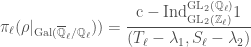
$\displaystyle \rho\otimes_{E} B(\rho_{p})\to \widehat{H}_{E,\Sigma}^{1}.$

Let us briefly discuss why this is true. Consider the smooth induced representation $\mathrm{c-Ind}_{\mathrm{GL}_{2}(\mathbb{Z}_{\ell})}^{{\mathrm{GL}_{2}(\mathbb{Q}_{\ell})}}1$ with compact support over $E$ . We have that $\mathrm{End}_{\mathrm{GL}_{2}(\mathbb{Q}_{\ell})}(\mathrm{c-Ind}_{\mathrm{GL}_{2}(\mathbb{Z}_{\ell})}^{{\mathrm{GL}_{2}(\mathbb{Q}_{\ell})}}1)\cong E[T_{\ell},S_{\ell}]$ . Now let $\pi_{\ell}$ be a smooth representation of $\mathrm{GL}_{2}(\mathbb{Q}_{\ell})$ over $E$ , and let $\lambda_{1}$ , $\lambda_{2}$ be in $E$ . We have

$\displaystyle \mathrm{Hom}_{\mathrm{GL}_{2}(\mathbb{Q}_{\ell})}\left(\frac{\mathrm{c-Ind}_{\mathrm{GL}_{2}(\mathbb{Z}_{\ell})}^{{\mathrm{GL}_{2}(\mathbb{Q}_{\ell})}}1}{(T_{\ell}-\lambda_{1},S_{\ell}-\lambda_{2})},\pi_{\ell}\right)=\pi_{\ell}^{\mathrm{GL}_{2}(\mathbb{Z}_{\ell})}[T_{\ell}-\lambda_{1},S_{\ell}-\lambda_{2}]$

Now let $\lambda:\mathbb{T}_{\Sigma}\to E$ be such that $\lambda(T_{\ell})=\mathrm{trace}(\rho(\mathrm{Frob}_{\ell}))$ and $\lambda(S_{\ell})=\ell^{-1}\mathrm{det}(\rho(\mathrm{Frob}_{\ell}))$ , for $\ell\not\in\Sigma$ . It follows from the (classical) local Langlands correspondence that

$\displaystyle \pi_{\ell}(\rho\vert_{\mathrm{Gal}(\overline{\mathbb{Q}}_{\ell}/\mathbb{Q}_{\ell}}))=\frac{\mathrm{c-Ind}_{\mathrm{GL}_{2}(\mathbb{Z}_{\ell})}^{{\mathrm{GL}_{2}(\mathbb{Q}_{\ell})}}1}{(T_{\ell}-\lambda_{1},S_{\ell}-\lambda_{2})}$

Let $\widehat{H}_{E,\Sigma}^{1}[\lambda]$ denote the subspace of $\widehat{H}_{E,\Sigma}^{1}$ on which $\mathbb{T}_{\Sigma}$ acts by $\lambda$ . The results that we have just discussed now tell us that the space

$\displaystyle \mathrm{Hom}_{\mathrm{Gal}(\overline{\mathbb{Q}}/\mathbb{Q})\times \mathrm{GL}_{2}(\mathbb{Q}_{p})\times\mathrm{GL}_{2}(\mathbb{A}_{f}^{\Sigma})}(\rho\otimes_{E} B(\rho_{p})\otimes'_{\ell\not\in\Sigma}\pi_{\ell}(\rho\vert_{\mathrm{Gal}(\overline{\mathbb{Q}}_{\ell}/\mathbb{Q}_{\ell})}),\widehat{H}_{E}^{1})$

is isomorphic to the space

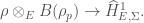
$\displaystyle \mathrm{Hom}_{\mathrm{Gal}(\overline{\mathbb{Q}}/\mathbb{Q})\times \mathrm{GL}_{2}(\mathbb{Q}_{p})}(\rho\otimes_{E} B(\rho_{p}),\widehat{H}_{E,\Sigma}^{1}[\lambda])$ .

Furthermore, it follows from Eichler-Shimura relations (which relate the action of $\mathrm{Gal}(\overline{\mathbb{Q}}/\mathbb{Q})$ and $\mathbb{T}_{\Sigma}$ on $\widehat{H}_{E,\Sigma}^{1}$ that the previous space is also isomorphic to

$\displaystyle \mathrm{Hom}_{\mathrm{Gal}(\overline{\mathbb{Q}}/\mathbb{Q})\times \mathrm{GL}_{2}(\mathbb{Q}_{p})}(\rho\otimes_{E} B(\rho_{p}),\widehat{H}_{E,\Sigma}^{1})$ .

Furthermore, for each of these isomorphisms, a morphism on one side of the isomorphism is a closed injection if and only if the corresponding morphism is also a closed injection. Therefore, as earlier stated, to show local-global compatibility it will be enough for us to show that a $\mathrm{Gal}(\overline{\mathbb{Q}}/\mathbb{Q})\times\mathrm{GL}_{2}(\mathbb{Q}_{p})$ -equivariant map $\rho\otimes_{E} B(\rho_{p})\to \widehat{H}_{E,\Sigma}^{1}$ exists.

Representations valued in a completion of the Hecke algebra

To show the existence of this map $\rho\otimes_{E} B(\rho_{p})\to \widehat{H}_{E,\Sigma}^{1}$ , we will construct a module that we shall denote by $X_{\mathcal{O}_{E}}$ . Before we can define this module though, we need to make some definitions involving the Hecke algebra, and representations valued in (completions of) this Hecke algebra.

Let $\overline{\rho}:\mathrm{Gal}(\overline{\mathbb{Q}}/\mathbb{Q})\to\mathrm{GL}_{2}(k_{E})$ be an absolutely irreducible odd continuous residual Galois representation. Let us suppose furthermore that $\overline{\rho}$ is modular.

Let $K_{\Sigma}$ be a compact open subgroup of $\prod_{\ell\in\Sigma}\mathrm{GL}_{2}(\mathbb{Q}_{\ell})$ . We let $\mathbb{T}(K_{\Sigma}\prod_{\ell\not\in\Sigma}\mathrm{GL}_{2}(\mathbb{Z}_{\ell}))_{\overline{\rho}}$ be the completion of $\mathbb{T}_{\Sigma}(K_{\Sigma}\prod_{\ell\not\in\Sigma}\mathrm{GL}_{2}(\mathbb{Z}_{\ell}))$ with respect to the maximal ideal generated by $\varpi$ , $T_{\ell}-\mathrm{tr}(\overline{\rho}(\mathrm{Frob}_{\ell})$ , and $S_{\ell}-\ell^{-1}\mathrm{det}(\overline{\rho}(\mathrm{Frob}_{\ell}))$ . 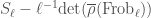We define

$\displaystyle \mathbb{T}_{\Sigma,\overline{\rho}}:=\varprojlim_{K_{\Sigma}}\mathbb{T}(K_{\Sigma}\prod_{\ell\not\in\Sigma}\mathrm{GL}_{2}(\mathbb{Q}_{\ell}))_{\overline{\rho}}.$

Since $\overline{\rho}$ is absolutely irreducible, for every compact open subgroup $K_{\Sigma}$ of $\pr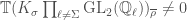od_{\ell\in\Sigma} \mathrm{GL}_{2}(\mathbb{Q}_{\ell})$ such that $\mathbb{T}(K_{\sigma}\prod_{\ell\neq\Sigma}\mathrm{GL}_{2}(\mathbb{Q}_{\ell}))_{\overline{\rho}}\neq 0$ the work of Carayol provides us with a unique continuous Galois module $\rho(\Sigma):\mathrm{Gal}(\overline{\mathbb{Q}}/\mathbb{Q})\to\mathrm{GL}_{2}(\mathbb{T}(K_{\sigma}\prod_{\ell\neq\Sigma}\mathrm{GL}_{2}(\mathbb{Q}_{\ell}))_{\overline{\rho}})$ unramified outside $\Sigma$ such that $\mathrm{trace}(\rho(K_{\Sigma})(\mathrm{Frob}_{\ell}))=T_{\ell}$ and $\mathrm{det}(\rho(K_{\Sigma})(\mathrm{Frob}_{\ell})=\ell S_{\ell}$ .

We define $\rho_{\Sigma}:=\varprojlim_{K_{\Sigma}}\rho(K_{\Sigma})$ . This is a deformation of $\overline{\rho}$ over the complete Noetherian local $\mathcal{O}_{E}$ -algebra $\mathbb{T}_{\Sigma,\overline{\rho}}$ (see also Galois Deformation Rings). After restriction to $\mathbb{Q}_{p}$ , we may also look at $\rho_{\Sigma}$ as a deformation of $\overline{\rho}_{p}$ .

Now let $\overline{\pi}_{p}$ is the representation associated to $\overline{\rho}_{p}$ by the mod p local Langlands correspondence. We also want to construct a deformation $\pi_{\Sigma}$ of $\overline{\pi}_{p}$ , that is related to $\rho_{\Sigma}$ by the p-adic local Langlands correspondence.

Let $R(\overline{\rho}_{p})$ be the deformation ring that represents the functor which assigns to a complete Noetherian local $\mathcal{O}_{E}$ -algebra the set of deformations of $\overline{\rho}_{p}$ over $A$ . We define $R(\overline{\rho}_{p})^{\mathrm{cris}}$ to be the the quotient of $R(\overline{\rho}_{p})$ by the intersection of all maximal ideals which are kernels of a map $R(\rho_{p})\to E'$ for some extension $E'$ of $E$ such that the representation over $E'$ obtained by base change from the universal representation over $R(\overline{\rho}_{p})$ is crystalline with distinct Hodge-Tate weights (see also p-adic Hodge Theory: An Overview).

Similarly, we have a deformation ring Let $R(\overline{\pi}_{p})$ that represents the functor which assigns to a complete Noetherian local $\mathcal{O}_{E}$ -algebra $A$ the set of deformations of $\overline{\rho}_{p}$ over $A$ . Recall that the p-adic local Langlands correspondence provides us with the Montreal functor $V$ from representations of $\mathrm{GL}_{2}(\mathbb{Q}_{p})$ to representations of $\mathrm{Gal}(\overline{\mathbb{Q}}_{p}/\mathbb{Q}_{p})$ , which means we have a map $R(\overline{\rho}_{p})\to R(\overline{\pi}_{p})$ . We let $R(\overline{\pi}_{p})^{\mathrm{det}}$ be the quotient of $R(\overline{\pi}_{p})$ parametrizing deformations $\pi_{p}$ of $\overline{\pi}_{p}$ whose central character corresponds to $\mathrm{det} V(\pi_{p})\varepsilon$ under local class field theory. We define

$R(\overline{\pi}_{p})^{\mathrm{cris}}:=R(\overline{\pi}_{p})\otimes_{R(\overline{\rho}_{p})}R(\overline{\rho}_{p})^{\mathrm{cris}}$

Now it turns out that the surjection $R(\overline{\pi}_{p})^{\mathrm{cris}}\twoheadrightarrow R(\overline{\rho}_{p})^{\mathrm{cris}}$ is actually an isomorphism. A consequence of this is that, if we have a complete Noetherian local $\mathcal{O}_{E}$ -algebra $T$ that is a quotient of $R(\overline{\rho}_{p})^{\mathrm{cris}}$ , any deformation $\rho_{p}$ of $\overline{\rho}_{p}$ over $T$ comes from a deformation $\pi_{p}$ of $\overline{\pi}_{p}$ via the Montreal functor $V$ .

Now all we need to do to construct $\pi_{\Sigma}$ is to find an appropriate complete Noetherian local $\mathcal{O}_{E}$ -algebra $T$ . We recall that $\rho_{\Sigma}$ is a deformation of $\overline{\rho}_{p}$ over $\mathbb{T}_{\Sigma,\overline{\rho}}$ , so we want to find $T$ inside of $\mathbb{T}_{\Sigma},\overline{\rho}$ , apply the discussion in the previous paragraph, and then we can extend scalars to obtain the deformation $\pi_{\Sigma}$ over $\mathbb{T}_{\Sigma,\overline{\rho}}$ . To do this we need to show to discuss crystalline classical maximal ideals, and show that they are Zariski dense inside $\mathbb{T}_{\Sigma,\overline{\rho}}$ (this fact will also be used again to achieve the goal we stated earlier of showing the existence of a map $\rho\otimes_{E} B(\rho_{p})\to \widehat{H}_{E,\Sigma}^{1}$ ).

We say that a maximal ideal $\mathfrak{p}$ of $\mathbb{T}_{\Sigma}$ is classical if the system of Hecke eigenvalues associated to $\mathbb{T}_{\Sigma}\to\mathbb{T}_{\Sigma}[1/p]/\mathfrak{p}$ comes from a cuspidal eigenform of weight $\geq 2$ .

Let $\mathfrak{p}$ be a classical maximal ideal of $\mathbb{T}_{\Sigma,\overline{\rho}}$ . Then we have a representation

$\displaystyle \rho_{\Sigma}\vert_{\mathrm{Gal}(\overline{\mathbb{Q}}_{p}/\mathbb{Q}_{p})}\otimes_{\mathbb{T}_{\Sigma,\overline{\rho}}} \mathbb{T}_{\Sigma,\overline{\rho}}[1/p]/\mathfrak{p}$

which is potentially semistable with distinct Hodge-Tate weights. We say that the classical maximal ideal $\mathfrak{p}$ is crystalline if the associated Galois representation is crystalline.

Let us now outline the argument showing that the crystalline classical maximal ideals are dense in $\mathbb{T}_{\Sigma,\overline{\rho}}$ . This is the same as the statement that the intersection of all crystalline classical maximal ideals is zero. And so our strategy will be to show that any element $t$ in this intersection acts by $0$ on $\widehat{H}_{E,\Sigma,\overline{\rho}}^{1}$ .

Let $K_{\Sigma}^{p}$ be a sufficiently small compact open subgroup of $\prod_{\ell\in\Sigma\setminus p}\mathrm{GL}_{2}(\mathbb{Q}_{\ell})$ . Then the $\mathrm{GL}_{2}(\mathbb{Z}_{p})$ -representation $\widehat{H}^{1}(K_{\Sigma}^{p}\prod_{\ell\not\in\Sigma}\mathrm{GL}_{2}(\mathbb{Z}_{p}))_{E,\overline{\rho}}$ is a topological direct factor of $\mathcal{C}(\mathrm{GL}_{2}(\mathbb{Z}),E)^{r}$ for some $r>0$ , where $\mathcal{C}(\mathrm{GL}_{2}(\mathbb{Z}),E)$ is the $\mathrm{GL}_{2}(\mathbb{Z}_{p})$ -representation provided by the continuous $E$ -valued functions on $\mathrm{GL}_{2}(\mathbb{Z}_{p})$ .

Now it happens that the polynomial functions of $\mathrm{GL}_{2}(\mathbb{Z}_{p})$ are dense inside the continuous functions $\mathcal{C}(\mathrm{GL}_{2}(\mathbb{Z}),E)$ . This implies that the vectors in $\mathcal{C}(\mathrm{GL}_{2}(\mathbb{Z}),E)^{r}$ for which $\mathrm{GL}_{2}(\mathbb{Z}_{p})$ acts algebraically are dense in $\mathcal{C}(\mathrm{GL}_{2}(\mathbb{Z}),E)^{r}$ . Since, by the previous paragraph, $\widehat{H}^{1}(K_{\Sigma}^{p}\prod_{\ell\not\in\Sigma}\mathrm{GL}_{2}(\mathbb{Z}_{p}))_{E,\overline{\rho}}$ is a topological direct factor of $\mathcal{C}(\mathrm{GL}_{2}(\mathbb{Z}),E)^{r}$ for $K_{\Sigma}^{p}$ sufficiently small, this implies that a similar result holds for $\widehat{H}^{1}(K_{\Sigma}^{p}\prod_{\ell\not\in\Sigma}\mathrm{GL}_{2}(\mathbb{Z}_{p}))_{E,\overline{\rho}}$ . Taking limits over $K_{\Sigma}^{p}$ , we obtain that the vectors in $\widehat{H}_{E,\Sigma,\overline{\rho}}^{1}$ for which $\mathrm{GL}_{2}(\mathbb{Z}_{p})$ acts by an algebraic representation of $\mathrm{GL}_{2}$ are dense in $\widehat{H}_{E,\Sigma,\overline{\rho}}^{1}$ .

If $\mathfrak{p}$ is a maximal ideal of $\mathbb{T}_{\Sigma,\overline{\rho}}$ , we write $\widehat{H}_{E,\Sigma,\overline{\rho}}^{1}[\mathfrak{p}]$ to denote the submodule of $\widehat{H}_{E,\Sigma,\overline{\rho}}^{1}$ annihilated by $\mathfrak{p}$ . We now have that $(\widehat{H}_{E,\Sigma,\overline{\rho}}^{1})^{\mathrm{alg}}$ is contained in $\oplus_{\mathfrak{p}}\widehat{H}_{E,\Sigma,\overline{\rho}}^{1}[\mathfrak{p}]$ , where the direct sum is over all classical maximal ideals of $\mathbb{T}_{\Sigma,\overline{\rho}}$ . Furthermore, the subrepresentation of $(\widehat{H}_{E,\Sigma,\overline{\rho}}^{1})^{\mathrm{alg}}$ generated by the vectors for which $\mathrm{GL}_{2}(\mathbb{Z}_{p})$ acts by an algebraic representation is contained in $\oplus_{\mathfrak{p}\in\mathcal{C}}\widehat{H}_{E,\Sigma,\overline{\rho}}^{1}[\mathfrak{p}]$ , where the direct sum is now over all crystalline classical maximal ideals of $\mathbb{T}_{\Sigma,\overline{\rho}}$ . Now it turns out that, if $\rho_{f}$ is the Galois representation associated to some cuspidal eigenform $f$ of weight $\geq 2$ , the representation $\pi_{p}(\rho_{f}\vert_{\mathrm{Gal}(\overline{\mathbb{Q}}_{p}/\mathbb{Q}_{p}))}$ contains a vector fixed under the action of $\mathrm{GL}_{2}(\mathbb{Z}_{p})$ if and only if $\rho_{f}\vert_{\mathrm{Gal}(\overline{\mathbb{Q}}_{p}/\mathbb{Q}_{p}))}$ is crystalline. If $t$ is an element in the intersection of all the crystalline classical maximal ideals, it annihilates $\oplus_{\mathfrak{p}\in\mathcal{C}}\widehat{H}_{E,\Sigma,\overline{\rho}}^{1}[\mathfrak{p}]$ , and therefore also the subrepresentation of $(\widehat{H}_{E,\Sigma,\overline{\rho}}^{1})^{\mathrm{alg}}$ generated by the vectors for which $\mathrm{GL}_{2}(\mathbb{Z}_{p})$ acts by an algebraic representation. But this subrepresentation is dense in $\widehat{H}_{E,\Sigma,\overline{\rho}}^{1}$ and by continuity $t$ acts by zero on $\widehat{H}_{E,\Sigma,\overline{\rho}}^{1}$ . This shows that the intersection of all the crystalline classical maximal ideals is zero and that they are Zariski dense in $\mathbb{T}_{\Sigma,\overline{\rho}}$ .

Since the crystalline classical maximal ideals are dense in in $\mathbb{T}_{\Sigma,\overline{\rho}}$ , we have that the map $R(\overline{\rho}_{p})\to\mathbb{T}_{\Sigma,\overline{\rho}}$ factors through $R(\overline{\rho}_{p})^{\mathrm{cris}}\to\mathbb{T}_{\Sigma,\overline{\rho}}$ . Now we find our complete Noetherian local $\mathcal{O}_{E}$ -algebra $T$ mentioned earlier as the image of the map $R(\overline{\rho}_{p})^{\mathrm{cris}}\to\mathbb{T}_{\Sigma,\overline{\rho}}$ , so that we can obtain a deformation $\pi_{p}$ of $\overline{\pi}_{p}$ that gives rise to $\rho_{p}$ via the Montreal functor $V$ . Then we extend scalars to $\mathbb{T}_{\Sigma,\overline{\rho}}$ to obtain $\pi_{\Sigma}$ .

Existence of the map

Now that we have the $\mathbb{T}(K_{\sigma}\prod_{\ell\neq\Sigma}\mathrm{GL}_{2}(\mathbb{Q}_{\ell}))_{\overline{\rho}}$ -valued representations $\rho_{\Sigma}$ and $\pi_{\Sigma}$ , we may now define the module $X_{\mathcal{O}_{E}}$ which as we said will help us prove the existence of a map $\rho\otimes_{E} B(\rho_{p})\to \widehat{H}_{E,\Sigma}^{1}$ . It is defined as follows:

$\displaystyle X_{\mathcal{O}_{E}}:=\mathrm{Hom}_{\mathbb{T}_{\Sigma,\overline{\rho}}[\mathrm{Gal}(\overline{\mathbb{Q}}/\mathbb{Q})\times\mathrm{GL}_{2}(\mathbb{Q}_{p})]}(\rho_{\Sigma}\otimes_{\mathbb{T}_{\Sigma,\overline{\rho}}}\pi_{\Sigma},\widehat{H}_{\mathcal{O}_{E}\Sigma,\overline{\rho}}^{1})$

Let $\mathfrak{p}$ be a maximal ideal of $\mathbb{T}_{\Sigma,\overline{\rho}}$ . We let $X_{E}[\mathfrak{p}]$ denote the set of elements of $X_{E}$ that are annihilated by the elements of $\mathfrak{p}$ . Our aim is to show that $X_{E}[\mathfrak{p}]\neq 0$ for all maximal ideals. As we shall show later, applying this to the maximal ideal generated by $\varpi$ , $T_{\ell}-\mathrm{tr}(\overline{\rho}(\mathrm{Frob}_{\ell})$ , and $S_{\ell}-\ell^{-1}\mathrm{det}(\overline{\rho}(\mathrm{Frob}_{\ell}))$ will give us our result. Our approach will be to show first that $X_{E}[\mathfrak{p}]\neq 0$ for “crystalline” maximal ideals, then, using the fact that the crystalline classical maximal ideals are Zariski dense in $\mathbb{T}_{\Sigma,\overline{\rho}}$ , show that this is true for all maximal ideals of $\mathbb{T}_{\Sigma,\overline{\rho}}$ .

Let $\mathfrak{p}$ be a crystalline classical maximal ideal of $\mathbb{T}_{\Sigma,\overline{\rho}}$ . Then $X_{E}[\mathfrak{p}]\neq 0$ . To show this, we choose some field $\widetilde{E}$ that contains $\mathbb{T}_{\Sigma,\overline{\rho}}[1/p]/\mathfrak{p}$ . Now recall again that we have

$\displaystyle \bigoplus_{k\geq 2,n\in\mathbb{Z}} \varinjlim_{K_{\Sigma}}H_{\mathrm{et}}^{1}(Y(K_{\Sigma}\prod_{\ell\neq \Sigma}\mathrm{GL}_{2}(\mathbb{Z}_{\ell}))\times_{\mathbb{Q}}\overline{\mathbb{Q}},\mathcal{F}_{k-2})\otimes_{\widetilde{E}}\mathrm{Sym}^{k-2}E'^{2})^{\vee}\otimes_{\widetilde{E}}\varepsilon^{n}\cong(\widehat{H}_{\widetilde{E},\Sigma}^{1})^{\mathrm{alg}}$

Now since $\widetilde{E}$ contains $\mathbb{T}_{\Sigma,\overline{\rho}}[1/p]/\mathfrak{p}$ , we find that inside $(\widehat{H}_{E',\Sigma}^{1})[\mathfrak{p}]$ there lies a tensor product of $\rho(\mathfrak{p})$ and some locally algebraic representation of $\mathrm{GL}_{2}(\mathbb{Q}_{p})$ . What the crystalline condition on $\mathfrak{p}$ does is it actually provides us with at most one equivalence class of invariant norms on this locally algebraic representation of $\mathrm{GL}_{2}(\mathbb{Q}_{p})$ , which must be the one induced by $(\widehat{H}_{\mathcal{O}_{\widetilde{E}},\Sigma}^{1})[\mathfrak{p}]$ on $(\widehat{H}_{\widetilde{E},\Sigma}^{1})[\mathfrak{p}]$ . It turns out that after completion, the representation of $\mathrm{GL}_{2}(\mathbb{Q}_{p})$ on the resulting p-adic Banach space is precisely $B(\rho(\mathfrak{p})\vert_{\mathrm{Gal}(\overline{\mathbb{Q}}_{p}/\mathbb{Q}_{p})})$ if $\rho(\mathfrak{p}\vert_{\mathrm{Gal}(\overline{\mathbb{Q}}_{p}/\mathbb{Q}_{p})})$ is irreducible, and a closed subrepresentation of $B(\rho(\mathfrak{p})\vert_{\mathrm{Gal}(\overline{\mathbb{Q}}_{p}/\mathbb{Q}_{p})})$ if $\rho(\mathfrak{p}\vert_{\mathrm{Gal}(\overline{\mathbb{Q}}_{p}/\mathbb{Q}_{p})})$ is reducible (here $\rho(\mathfrak{p})=\rho_{\Sigma}\otimes_{\mathbb{T}_{\Sigma,\overline{\rho}}}\mathbb{T}_{\Sigma,\overline{\rho}}[1/p]/\mathfrak{p}$ and $B(\rho(\mathfrak{p})\vert_{\mathrm{Gal}(\overline{\mathbb{Q}}_{p}/\mathbb{Q}_{p})})=\pi_{\Sigma}\otimes_{\mathbb{T}_{\Sigma,\overline{\rho}}}\mathbb{T}_{\Sigma,\overline{\rho}}[1/p]/\mathfrak{p}$ , and these two correspond to each other under the p-adic local Langlands correspondence).

Now we know that $X_{E}[\mathfrak{p}]\neq 0$ if $\mathfrak{p}$ is a crystalline classical maximal ideal. Now we want to extend this to all the maximal ideals of $\mathbb{T}_{\Sigma,\overline{\rho}}[1/p]$ by making use of the fact that the set of crystalline classical maximal ideals is Zariski dense inside $\mathbb{T}_{\Sigma,\overline{\rho}}[1/p]$ .

The idea is that, if $X_{E}[\mathfrak{p}]\neq 0$ for all maximal ideals $\widetilde{\mathfrak{p}}$ that belong to some set $\mathcal{E}$ that is Zariski dense in $\mathbb{T}_{\Sigma,\overline{\rho}}[1/p]$ , then $X_{E}[\mathfrak{p}]\neq 0$ for all maximal ideals $\mathfrak{p}$ in $\mathbb{T}_{\Sigma,\overline{\rho}}[1/p]$ . Let us consider first the simpler case of a module $M$ of finite type over $\mathbb{T}_{\Sigma,\overline{\rho}}[1/p]$ . We want to show that if $M/\widetilde{\mathfrak{p}}\neq 0$ for all $\widetilde{\mathfrak{p}}\in \mathcal{E}$ then $M/\mathfrak{p}\neq 0$ for all maximal ideals $\mathfrak{p}$ in $\mathbb{T}_{\Sigma,\overline{\rho}}[1/p]$ .

Since $\mathfrak{p}$ is maximal, $\mathbb{T}_{\Sigma,\overline{\rho}}[1/p]/\mathfrak{p}$ is a field, and $\mathbb{T}_{\Sigma,\overline{\rho}}[1/p]/\mathfrak{p}$ acts faithfully on $M/\mathfrak{p}M$ . If some element $t\in\mathbb{T}_{\Sigma,\overline{\rho}}[1/p]$ acts by zero on $M$ it must act by zero on $M/\mathfrak{p}M$ for all $\mathfrak{p}$ . If $M/\mathfrak{p}M\neq 0$ for all $\widetilde{\mathfrak{p}}\in \mathcal{E}$ , then this element $t$ must be in the intersection of all the $\widetilde{\mathfrak{p}}$ in $\mathcal{E}$ , but since $\mathcal{E}$ is Zariski dense in $\mathbb{T}_{\Sigma,\overline{\rho}}[1/p]$ , this intersection is zero and $t$ has to be zero.

Suppose for the sake of contradiction that $M/\mathfrak{p}M\neq 0$ for all $\widetilde{\mathfrak{p}}\in \mathcal{E}$ but $M/\mathfrak{p}M=0$ for some maximal ideal $\mathfrak{p}$ in $\mathbb{T}_{\Sigma,\overline{\rho}}[1/p]$ . Then Nakayama’s lemma says that there exists some nonzero element $t\in\mathbb{T}_{\Sigma,\overline{\rho}}[1/p]$ such that $tM=0$ . But this contradicts the above paragraph, so we must have $M/\mathfrak{p}M\neq 0$ for all maximal ideals $\mathfrak{p}$ in $\mathbb{T}_{\Sigma,\overline{\rho}}[1/p]$ .

Now let $K_{\Sigma}^{p}$ be a compact open subgroup of $\prod_{\ell\not\in\Sigma}\mathrm{GL}_{2}(\mathbb{Q}_{\ell})$ , and let $X_{\mathcal{O}_{E}}^{K_{\Sigma}^{p}}$ be defined similarly to $X_{\mathcal{O}_{E}}$ but with $\widehat{H}_{\mathcal{O}_{E}}^{1}(K_{\Sigma}^{p})$ in place of $\widehat{H}_{\mathcal{O}_{E}}^{1}$ . We apply the above argument to $\mathrm{Hom}_{\mathcal{O_{E}}}(X_{\mathcal{O}_{E}}^{K_{\Sigma}^{p}},\mathcal{O}_{E})\otimes_{\mathcal{O}_{E}} E$ , which is a $\mathbb{T}_{\Sigma,\overline{\rho}}[1/p]$ -module of finite type. Then it is a property of $X_{\mathcal{O}_{E}}$ (which is $\varinjlim_{K_{\Sigma}^{p}}X_{\mathcal{O}_{E}}^{K_{\Sigma}^{p}}$ ) that $X_{\mathcal{O}_{E}}[\mathfrak{p}]\neq 0$ if $X_{\mathcal{O}_{E}}^{K_{\Sigma}^{p}}[\mathfrak{p}]\neq 0$ for sufficiently small $K_{\Sigma}^{p}$ .

Now that we know that $X_{\mathcal{O}_{E}}[\mathfrak{p}]\neq 0$ for all maximal ideals $\mathfrak{p}$ of $\mathbb{T}_{\Sigma,\overline{\rho}}[1/p]$ , we apply this to the particular maximal ideal $\mathfrak{p}_{\rho}$ generated by $T_{\ell}-\mathrm{trace}(\rho(\mathrm{Frob}_{\ell}))$ and $S_{\ell}-\ell^{-1}\mathrm{det}(\rho(\mathrm{Frob}_{\ell}))$ . But we have

$\displaystyle X_{\mathcal{O}_{E}}[\mathfrak{p}_{\rho}]\otimes E=\mathrm{Hom}_{\mathbb{T}_{\Sigma,\overline{\rho}}/\mathfrak{p_{\rho}}[\mathrm{Gal}(\overline{\mathbb{Q}}/\mathbb{Q})\times\mathrm{GL}_{2}(\mathbb{Q}_{p})]}(\rho(\mathfrak{p}_{\rho})\otimes_{\mathbb{T}_{\Sigma,\overline{\rho}}/\mathfrak{p}_{\rho}}B(\rho(\mathfrak{p}_{\rho})\vert_{\mathrm{Gal}(\overline{\mathbb{Q}}_{p}/\mathbb{Q}_{p})}),\widehat{H}_{E,\Sigma,\overline{\rho}}^{1}[\mathfrak{p}_{\rho}])$

where again $\rho(\mathfrak{p}_{\rho})=\rho_{\Sigma}\otimes_{\mathbb{T}_{\Sigma,\overline{\rho}}}\mathbb{T}_{\Sigma,\overline{\rho}}[1/p]/\mathfrak{p}_{\rho}$ and $B(\rho(\mathfrak{p}_{\rho})\vert_{\mathrm{Gal}(\overline{\mathbb{Q}}_{p}/\mathbb{Q}_{p})})=\pi_{\Sigma}\otimes_{\mathbb{T}_{\Sigma,\overline{\rho}}}\mathbb{T}_{\Sigma,\overline{\rho}}[1/p]/\mathfrak{p}_{\rho}$ . Since we have just shown that the left-hand side of the above isomorphism is nonzero, then so must the right hand-side, which means there is map $\rho\otimes_{E} B(\rho_{p})\to \widehat{H}_{E,\Sigma}^{1}$ .

Furthermore this map is a closed injection if $\rho_{p}$ is not a direct sum of two characters or an extension of a character by itself. In the case that $\rho_{p}$ is absolutely irreducible, this follows from the fact that $B(\rho_{p})$ is topologically irreducible and admissible. If $\rho_{p}$ is reducible and indecomposable, then $B(\rho_{p})$ is also reducible and indecomposable and one needs to show that a nonzero morphism cannot be factorized by a strict quotient of $B(\rho_{p})$ . We leave further discussion of these to the references.

Application to the Fontaine-Mazur conjecture

Let us now discuss the application of local-global compatibility to (a special case of) the Fontaine-Mazur conjecture, whose statement is as follows.

Let $\rho:\mathrm{Gal}(\overline{\mathbb{Q}}/\mathbb{Q})\to\mathrm{GL}_{2}(E)$ be an absolutely irreducible odd continuous p-adic Galois representation, unramified at all but finitely many places, and whose restriction to $\mathrm{Gal}(\overline{\mathbb{Q}}_{p}/\mathbb{Q}_{p})$ is potentially semistable with distinct Hodge-Tate weights. Then the Fontaine-Mazur conjecture states that there exists some cuspidal eigenform $f$ of weight $\geq 2$ such that $\rho$ is the twist of $\rho_{f}$ (the Galois representation associated to $f$ ) by some character.

The Fontaine-Mazur conjecture is also often stated in the following manner. Let $\rho$ be as in the previous paragraph. Then $\rho$ can be obtained as the subquotient of the etale cohomology of some variety. This statement in fact follows from the previous one, because if $\rho_{f}$ is a Galois representation obtained from some cuspidal eigenform $f$ of weight $\geq 2$ , then it may be found as the subquotient of the etale cohomology of what is known as a Kuga-Sato variety.

Now let us discuss how local-global compatibility figures into the proof (due to Matthew Emerton) of a special case of the Fontaine-Mazur conjecture. This special case is when $p>2$ and we have the restriction of the corresponding residual Galois representation $\overline{\rho}$ to $\mathrm{Gal}(\overline{\mathbb{Q}}/\mathbb{Q}(\zeta_{p}))$ is absolutely irreducible, and the restriction of $\overline{\rho}$ to $\mathrm{Gal}(\overline{\mathbb{Q}}_{p}/\mathbb{Q}_{p})$ is not isomorphic to a Galois representation of the form $\begin{pmatrix}1&0\\0&\overline{\epsilon}\end{pmatrix}$ twisted by a character for $p>3$ , or $\begin{pmatrix}1&*\\0&\overline{\epsilon}\end{pmatrix}$ twisted by a character for $p=3$ .

In this case it follows from the work of Böckle, Diamond-Flach-Guo, Khare-Wintenberger, and Kisin that $\rho$ is promodular. Then the local-global compatibility that we have discussed tells us that we have a closed injective map $B(\rho_{p})\hookrightarrow \mathrm{Hom}_{\mathrm{Gal}(\overline{\mathbb{Q}}/\mathbb{Q})}(\rho,\widehat{H}_{E}^{1})$ . The condition of the restriction $\rho_{p}$ being potentially semistable with distinct Hodge-Tate weights guarantees that $B(\rho_{p})^{\mathrm{alg}}\neq 0$ (here $B(\rho_{p})^{\mathrm{alg}}$ is defined exactly the same as $(\widehat{H}_{E,\Sigma}^{1})^{\mathrm{alg}}$ except with $B(\rho_{p})$ in place of $(\widehat{H}_{E,\Sigma}^{1})$ ). This follows from the compatibility of the p-adic local Langlands correspondence and the “classical” local Langlands correspondence, which says that if $\rho_{p}$ is potentially semistable with distinct Hodge-Tate weights $a<b$ then we have the following isomorphism:

$\displaystyle \mathrm{det}^{a+1}\otimes_{E}\mathrm{Sym}^{b-a-1}E^{2}\otimes_{E}\pi_{p}(\rho_{p})\xrightarrow{\sim}B(\rho_{p})^{\mathrm{alg}}$

The closed injective map $B(\rho_{p})\hookrightarrow \mathrm{Hom}_{\mathrm{Gal}(\overline{\mathbb{Q}}/\mathbb{Q})}(\rho,\widehat{H}_{E}^{1})$ then tells us that, since $B(\rho_{p})^{\mathrm{alg}}\neq 0$ , we must have $(\widehat{H}_{E,\Sigma}^{1})^{\mathrm{alg}}\neq 0$ as well. But we have the isomorphism

and the Galois representations that show up on the left hand side of this isomorphism are associated to cuspidal eigenforms of weights $k\geq 2$ . This completes our sketch of the proof of the special case of the Fontaine-Mazur conjecture.

We have discussed here the ideas involved in Emerton’s proof of a special case of the Fontaine-Mazur conjecture. There is also another proof due to Mark Kisin that makes use of a different approach, namely, ideas related to the Breuil-Mezard conjecture (a version of which was briefly discussed in Moduli Stacks of (phi, Gamma)-modules) and the method of “patching” (originally developed as part of the approach to proving Fermat’s Last Theorem). This approach will be discussed in future posts on this blog.

References:

Correspondance de Langlands p-adique, compatibilité local-global et applications by Christophe Breuil

Local-global compatibility in the p-adic Langlands programme for GL_2/Q by Matthew Emerton

A local-global compatibility conjecture in the p-adic Langlands programme for GL_2/Q by Matthew Emerton

Completed cohomology and the p-adic Langlands program by Matthew Emerton

The Breuil-Schneider conjecture, a survey by Claus M. Sorensen

Siegel modular forms

December 14, 2021December 14, 2021 / Anton Hilado / 2 Comments

In Modular Forms we introduced modular forms as certain holomorphic functions on the upper half-plane following certain transformation properties with respect to the action of the group $\mathrm{SL}_{2}(\mathbb{Z})$ (or more generally its congruence subgroups). We also saw that they are sections of certain sheaves on the compactified moduli space of elliptic curves, possibly together with extra structure, such as a basis of $N$ -torsion, a point of order $N$ , or a cyclic subgroup of order $N$ (see also The Moduli Space of Elliptic Curves).

In this post we shall introduce a higher-dimensional generalization of this idea. Namely, we shall introduce Siegel modular forms, which are to principally polarized abelian varieties as the usual (also called elliptic) modular forms are to elliptic curves.

Let us follow the same approach that we used to introduce modular forms, as certain functions on the upper half-space with certain transformation properties. Therefore the first thing we will need is a higher-dimensional analogue of the upper half-space.

The Siegel upper half-space of degree $g$ (or genus $g$ ), denoted $\mathcal{H}_{g}$ is the set of all $g\times g$ symmetric matrices whose entries are complex numbers with a positive imaginary part. If $g=1$ , then this is the same as the usual upper half-space.

Now we need the analogue of the transformation properties of an elliptic modular form under the modular group $\mathrm{SL}_{2}(\mathbb{Z})$ . We recall that the action of $\mathrm{SL}_{2}(\mathbb{Z})$ on the upper half-plane was inherited from the action of $\mathrm{SL}_{2}(\mathbb{R})$ via Mobius transformations. If $\begin{pmatrix}a&b\\c&d\end{pmatrix}$ is an element of $\gamma=\mathrm{SL}_{2}(\mathbb{R})$ , then it maps a point $\tau$ on the upper half-plane to $\displaystyle \gamma(z)=\frac{a\tau+b}{c\tau+d}$ . Then we define a modular form of weight $k$ to be a holomorphic function $f:\mathcal{H}\to\mathbb{C}$ such that $f(\gamma(\tau))=(c\tau+d)^{k}f(\tau)$ and such that $f$ is holomorphic at infinity (it is bounded as the imaginary part of $\tau$ approaches infinity).

For Siegel modular form, our group will be the Siegel modular group $\mathrm{Sp}_{2g}(\mathbb{Z})$ , which is a subgroup of the symplectic group $\mathrm{Sp}_{2g}(\mathbb{R})$ . The elements of the symplectic group are $2g\times 2g$ real matrices which can be written in the form $\begin{pmatrix}A&B\\C&D\end{pmatrix}$ where $A$ , $B$ , $C$ , and $D$ are $g\times g$ real matrices satisfying $AB^{T}=BA^{T}$ , $CD^{T}=DC^{T}$ , and $AD^{T}-DC^{T}=I_{g}$ , where the superscript ${}^{T}$ means taking the transpose and $I_{g}$ is the $g\times g$ identity matrix. Note that if $g=1$ , then the first two conditions are automatically satisfied while the third condition says that the determinant of the matrix must be $1$ . Therefore $\mathrm{Sp}_{2}(\mathbb{R})=\mathrm{SL}_{2}(\mathbb{R})$ .

Now let $\tau$ be an element of the Siegel upper half-plane $\mathcal{H}_{g}$ . Note that $\tau$ is now a $g\times g$ matrix. An element $\gamma$ of $\mathrm{Sp}_{2g}(\mathbb{R})$ sends $\tau$ to the element

$\gamma(\tau)=(A\tau+B)(C\tau+D)^{-1}$ .

We are almost ready to define Siegel modular forms. Although we may define Siegel modular forms as being complex-valued just like elliptic modular forms, and they are in themselves worthwhile objects of study, it is sometimes more natural to consider Siegel modular forms as being vector-valued. This arises for example when we want to obtain Siegel modular forms as sections of the Hodge bundle, which is the pushforward of the sheaf of relative differentials of the universal principally polarized abelian variety over $\mathbb{C}$ on the moduli space of principally polarized abelian varieties over $\mathbb{C}$ (which is obtained as the quotient of $\mathcal{H}_{2g}$ by $\mathrm{Sp}_{2g}(\mathbb{Z})$ ).

Let $V$ be a finite-dimensional vector space over $\mathbb{C}$ , and let $\rho:\mathrm{GL}_{g}(\mathbb{C})\to \mathrm{GL}(V)$ be a representation of $\mathrm{GL}_{g}(\mathbb{C})$ on $V$ . A Siegel modular form of weight $\rho$ is a holomorphic function $f:\mathcal{H}_{g}\to V$ such that

$\displaystyle f(\gamma(\tau))=\rho(C\tau+D)f(\tau)$

for any $g\in\mathrm{SL}_{2}(\mathbb{Z})$ , and which is holomorphic at infinity if $g=1$ . If $g>1$ , the holomorphicity at infinity is automatically taken care of by what is known as Kocher’s principle.

In the special case that $V=\mathbb{C}$ , and $\rho$ is given by taking powers of the determinant, i.e. our Siegel modular form is a holomorphic function $f:\mathcal{H}\to\mathbb{C}$ such that

$f(\gamma(\tau))=\mathrm{det}(C\tau+D)^{k}f(\tau)$

then we say that our Siegel modular form is a classical Siegel modular form. Note that a classical Siegel modular form of degree $1$ is an elliptic modular form.

We may also consider Siegel modular forms for congruence subgroups $\Gamma(N)$ of $\mathrm{Sp}_{2g}(\mathbb{Z})$ , where $\Gamma(N)$ is the subgroup of $\mathrm{Sp}_{2g}(\mathbb{Z})$ consisting of elements that become the identity matrix after reduction mod $N$ .

The theory of Siegel modular forms is more complicated than the theory of elliptic modular forms, but we may use the latter to guide our study of the former. For instance, we may want to consider the Fourier expansion of Siegel modular forms. We may also want to consider its Hecke algebra (see also Hecke Operators). There are also analogues of important examples of elliptic modular forms, such as the Eisenstein series or the discriminant, for Siegel modular forms. We may also use elliptic modular forms to construct explicit examples of Siegel modular forms (a process known as lifting). All these and more will hopefully be discussed in future posts on this blog.

References:

Siegel modular form on Wikipedia

Siegel upper half-space on Wikipedia

Siegel modular variety on Wikipedia

Symplectic group on Wikipedia

Siegel modular forms by Gerard van der Greer

Automorphic Forms

September 15, 2021September 15, 2021 / Anton Hilado / 2 Comments

An automorphic form is a kind of function of the adelic points (see also Adeles and Ideles) of a reductive group (see also Reductive Groups Part I: Over Algebraically Closed Fields), that can be used to investigate its representation theory. Choosing an important kind of function of a group that will be helpful in investigating its representation theory was also discussed in Representation Theory and Fourier Analysis, where we found the square-integrable functions on the circle to be useful in studying its representations (or that of the real line) since it decomposed into a direct sum of irreducible representations. In fact, the cuspidal automorphic forms we will introduce later on in this post will also have this property (called semisimple) of decomposing into a direct sum of irreducible representations.

Remark: We have briefly mentioned, in the unramified case, cuspidal automorphic forms as certain functions on $\mathrm{Bun}_{G}$ in The Global Langlands Correspondence for Function Fields over a Finite Field. The function field (over a finite field) version of the cuspidal automorphic forms we define here are actually obtained as linear combinations of translates of such functions hence why it is enough to study them. In this post, we will discuss automorphic forms in more detail, beginning with the version over the field of rational numbers before generalizing to more general global fields.

Defining modular forms as functions on $\mathrm{GL}_{2}(\mathbb{A})$

In a way, automorphic forms can also generalize modular forms (see also Modular Forms), and this will give us a way to connect the two theories. We shall take this route first and recast modular forms in a new language – instead of functions on the upper half-plane, we shall now look at them as functions on the group $\mathrm{GL}_{2}(\mathbb{A})$ (here $\mathbb{A}$ denotes the adeles of $\mathbb{Q}$ ).

Let $K_{f}$ be a compact open subgroup of $\mathrm{GL}_{2}(\mathbb{A}_{f})$ whose elements all have determinants in $\widehat{\mathbb{Z}}^{\times}$ . Here $\mathbb{A}_{f}$ stands for the finite adeles, which are defined in the same way as the adeles, except we don’t include the infinite primes in the restricted product. We have that

$\displaystyle \mathrm{GL_{2}}(\mathbb{A})=\mathrm{GL_{2}}(\mathbb{Q})\mathrm{GL}_{2}(\mathbb{R})^{+}K_{f}$

where $\mathrm{GL}_{2}(\mathbb{R})^{+}$ is the subgroup of $\mathrm{GL}_{2}(\mathbb{R})$ consisting of elements that have positive determinant. Now let us take the double quotient $\mathrm{GL_{2}}(\mathbb{Q})\backslash\mathrm{GL}_{2}(\mathbb{A})/K_{f}$ . By the above expression for $\mathrm{GL}_{2}(\mathbb{A})$ as a product, we have

$\displaystyle \mathrm{GL_{2}}(\mathbb{Q})\backslash\mathrm{GL}_{2}(\mathbb{A})/K_{f}\simeq \Gamma\backslash\mathrm{GL_{2}}(\mathbb{R})$

where $\Gamma$ is the subgroup of $\mathrm{GL}_{2}(\mathbb{R})$ given by projecting $\mathrm{GL}_{2}(\mathbb{Q})\cap \mathrm{GL}_{2}(\mathbb{R})^{+}K_{f}$ into its archimedean component. Now suppose we are in the special case that $K_{f}$ is given by $\displaystyle \prod_{p} \mathrm{GL}_{2}(\mathbb{Z}_{p})$ . Then it turns out that $\Gamma$ is just $\mathrm{SL}_{2}(\mathbb{Z})$ ! Using appropriate choices of $K_{f}$ , we can also obtain congruence subgroups such as $\Gamma_{0}(N)$ (see also Modular Forms).

The group $\mathrm{GL}_{2}(\mathbb{R})^{+}$ acts on the upper half-plane by fractional linear transformations, i.e. if we have $\displaystyle g_{\infty}=\begin{pmatrix} a & b \\ c & d \end{pmatrix}\in\mathrm{GL}_{2}(\mathbb{R})^{+}$ , then $g_{\infty}$ sends $\tau$ in the upper half-plane to $\displaystyle g_{\infty}(\tau)=\frac{az+b}{cz+d}$ . Let

$\displaystyle j(g_{\infty},\tau)=\mathrm{det}(g_{\infty})^{-\frac{1}{2}}(c\tau+d)$ .

Now given a modular form $f$ of weight $m$ and level $\Gamma_{0}(N)$ , we may associate to it a function $\phi_{\infty}(g_{\infty})$ on $\mathrm{GL}_{2}(\mathbb{R})^{+}$ as follows:

$\displaystyle f\mapsto \phi_{\infty}(g_{\infty})=f(g_{\infty}(i))j(g_{\infty},i)^{-m}$

We can also go the other way, recovering $f$ from such a $\phi_{\infty}$ :

$\displaystyle \phi_{\infty}\mapsto f(g_{\infty}(i))=\phi_{\infty}(g_{\infty})j(g_{\infty},i)^{m}$

for any $g_{\infty}$ such that $g_{\infty}(i)=\tau$ . Ultimately we want a function $\phi$ on $\mathrm{GL}_{2}(\mathbb{A})$ , and we achieve this by setting $\phi(g)=\phi(\gamma g_{\infty} k_{f})$ to just have the same value as $\phi_{\infty}(g_{\infty})$ .

Translating properties of modular forms into properties of functions on $\mathrm{GL}_{2}(\mathbb{A})$

Invariance under $\mathrm{GL}_{2}(\mathbb{Q}$ and $K_{f}$

Now we want to know what properties $\phi$ must have, so that we can determine which functions on $\mathrm{GL}_{2}(\mathbb{A})$ come from modular forms. We have just seen that we must have

$\displaystyle \phi(g)=\phi(\gamma g_{\infty} k_{f})=\phi_{\infty}(g)$ .

The action of $Z_{\infty}^{+}$ and $K_{\infty}^{+}$

Let us now consider the action of the center of $\mathrm{GL}_{2}(\mathbb{R})^{+}$ (which we denote by $Z_{\infty}$ ) and the action of $\mathrm{SO}(2)$ , which is a maximal compact subgroup of $\mathrm{GL}_{2}(\mathbb{R})^{+}$ (and therefore we shall also denote it by $K_{\infty})^{+}$ . The center $Z_{\infty}$ is composed of the matrices of the form $z_{\infty}$ times the identity matrix, and it acts trivially on the upper half-plane. Therefore we will have

$\displaystyle j(z_{\infty}g_{\infty},\tau)=\mathrm{sgn}(z_{\infty})\mathrm{det}(g_{\infty})^{-\frac{1}{2}}(c\tau+d)$

Now for the maximal compact subgroup $K_{\infty}^{+}$ . As previously mentioned, this is the group $\mathrm{SO}(2)$ , and may be expressed as matrices of the form

$\displaystyle k_{\theta}=\begin{pmatrix}\mathrm{cos}(\theta) & \mathrm{sin}(\theta)\\-\mathrm{sin}(\theta) & \mathrm{cos}(\theta)\end{pmatrix}$ .

Then in the action of $\mathrm{GL}_{2}(\mathbb{R})^{+}$ on the upper half-plane, $Z_{\infty}K_{\infty}^{+}$ is the stabilizer of $i$ . We will also have

$\displaystyle j(z_{\infty}k_{\theta},i)=\mathrm{sgn}(z_{\infty})e^{i\theta}$

This leads us to the second property our function $\phi$ must satisfy. First we consider $\phi_{\infty}$ . For $z_{\infty}k_{\theta}\in Z_{\infty}K_{\infty}^{+}$ , we must have

$\displaystyle \phi_{\infty}(g_{\infty}z_{\infty}k_{\theta})=\phi_{\infty}(g_{\infty})\mathrm{sgn}(z)^{m}(e^{i\theta})^{m}$ .

Note the appearance of the weight $m$ . Now when we extend this function $\phi_{\infty}$ on $\mathrm{GL}_{2}(\mathbb{R})^{+}$ to a function $\phi$ on $\mathrm{GL}_{2}(\mathbb{A})$ , we must replace $Z_{\infty}$ by its connected component $Z_{\infty}^{+}$ .

Holomorphicity and the action of the Lie algebra

Next we must translate the property that the modular form $f$ is holomorphic into a property of $\phi$ . For this we shall introduce certain “raising” and “lowering” operators.

Let $\mathfrak{g}_{0}$ be the (real) Lie algebra of $\mathrm{GL}_{2}(\mathbb{R})^{+}$ . An element $X\in\mathfrak{g}_{0}$ acts on the space of smooth functions on $\mathrm{GL}_{2}(\mathbb{R})^{+}$ as follows:

$\displaystyle X\phi(g_{\infty})=\frac{d}{dt}\phi(g_{\infty}\mathrm{exp}(tX))\bigg\vert_{t=0}$

We can extend this to an action of the complexified Lie algebra $\mathfrak{g}$ , defined to be $\mathfrak{g}\otimes_{\mathbb{R}} \mathbb{C}$ , by setting

$\displaystyle (X+iY)\phi=X\phi+iY\phi$

We now look at two special elements of $\mathfrak{g}$ . They are

$\displaystyle X_{+}=\frac{1}{2}\begin{pmatrix}1 & i\\i & -1\end{pmatrix}$

and

$\displaystyle X_{-}=\frac{1}{2}\begin{pmatrix}1 & -i\\-i & -1\end{pmatrix}$ .

Let us now look at how these special elements act on the smooth functions on $\mathrm{GL}_{2}(\mathbb{R})^{+}$ . We have

$\displaystyle X_{+}\phi(g_{\infty}k_{\theta})=\phi(g_{\infty})(e^{i\theta})^{m+2}$

and

$\displaystyle X_{-}\phi(g_{\infty}k_{\theta})=\phi(g_{\infty})(e^{i\theta})^{m-2}$

In other words, the action of $X_{+}$ raises the weight by $2$ , while the action of $X_{-}$ lowers the weight by $2$ . Now it turns out that the condition that the function $f$ on the upper half-plane is holomorphic is the same condition as the function $\phi$ on $\mathrm{GL}_{2}(\mathbb{R})^{+}$ satisfying $X_{-}\phi=0$ !

Holomorphicity at the cusps

Now we have expressed the holomorphicity of our modular form $f$ as a condition on our function $\phi$ on $\mathrm{GL}_{2}(\mathbb{A})$ . However not only do we want our modular forms to be holomorphic on the upper half-plane, we also want them to be “holomorphic at the cusps”, i.e. they do not go to infinity at the cusps. This is going to be accomplished by requiring the function $g_{\infty}\mapsto \phi(g_{\infty}g_{f})$ to be “slowly increasing” for all $g_{f}\in\mathrm{GL}_{2}(\mathbb{A}_{f})$ . This means that for all $g_{f}\in\mathrm{GL}_{2}(\mathbb{A}_{f})$ , we have

$\displaystyle \vert \phi(g_{\infty}g_{f})\geq C\Vert g_{\infty}\Vert^{N}$

where $C$ and $N$ are some positive constants and the norm on the right-hand side is given by, for $g_{\infty}=\begin{pmatrix}a & b\\c & d\end{pmatrix}$ ,

$\displaystyle \Vert \phi(g_{\infty}g_{f})\Vert=(a^{2}+b^{2}+c^{2}+d^{2})(1+\mathrm{det}(g_{\infty}^{-2}))=\mathrm{Tr}(g_{\infty}^{T}g_{\infty})+\mathrm{Tr}((g_{\infty}^{-1})^{T}g_{\infty}^{-1})$ .

Summary of the properties

Let us summarize now the properties we want our function $\phi$ to have in order that it come from a modular form $f$ :

For all $\gamma\in\mathrm{GL}_{2}(\mathbb{Q})$ , we have $\phi(\gamma g)=\phi(g)$ .
For all $k_{f}\in K_{f}$ , we have $\phi(gk_{f})=\phi(g)$ .
For all $g_{f}\in\mathrm{GL}_{2}(\mathbb{A}_{f})$ , the function $g_{\infty}\mapsto \phi(g_{\infty}g_{f})$ is smooth.
For all $k_{\theta}\in K_{\infty}$ we have $\phi(gk_{\theta})=\phi(g)e^{i\theta}$ .
The function $\phi$ is invariant under $Z_{\infty}^{+}$ .
We have $\displaystyle X_{-}\phi=0$ .
The function given by $g_{\infty}\mapsto\phi(g_{\infty}g_{f})$ is slowly increasing.

Cuspidality

Now let us consider the case where $f$ is a cusp form. We want to translate the cuspidality condition to a condition on $\phi$ , and we do this by noting that this means that the Fourier expansion of $f$ has no constant term. Given that Fourier coefficients can be expressed using Fourier transforms, we make use of the measure theory on the adeles to express this cuspidality condition as

$\displaystyle \int_{\mathbb{Q}\setminus\mathbb{A}}\phi\left(\begin{pmatrix}1 & x\\0&1\end{pmatrix}\right)dx=0$ .

Automorphic forms

We have now defined modular forms as functions on $\mathrm{GL}_{2}(\mathbb{A})$ , and enumerated some of their important properties. Modular forms, as functions on $\mathrm{GL}_{2}(\mathbb{A})$ , turn out to be merely be specific examples of more general functions on $\mathrm{GL}_{2}(\mathbb{A})$ that satisfy similar, but more relaxed, properties. These are the automorphic forms.

The first few properties are the same, for instance for all $\gamma\in\mathrm{GL}_{2}(\mathbb{Q})$ , we want $\phi(\gamma g)=\phi(g)$ , and for all $k_{f}\in K_{f}$ , where $K_{f}$ is a compact subgroup of $\mathrm{GL}_{2}(\mathbb{A}_{f})$ , we want $\phi(g k)=\phi(g)$ . We will also want the function given by $g_{\infty}\mapsto \phi(g_{\infty}g_{f})$ to be smooth for all $g_{f}\in\mathrm{GL}_{2}(\mathbb{A}_{f})$ .

What we want to relax a little bit is the conditions on the actions of $K_{\infty}$ , $Z_{\infty}^{+}$ , and the Lie algebra $\mathfrak{g}$ , in that we want the space we get by having them act on some function $\phi$ to be finite-dimensional. Instead of looking at the action of the Lie algebra $\mathfrak{g}$ , it is often convenient to instead look at the action of its universal enveloping algebra $U(\mathfrak{g})$ . The universal enveloping algebra is an honest to goodness associative algebra that contains the Lie algebra (and is in fact generated by its elements) such that the commutator of the universal enveloping algebra gives the Lie bracket of the Lie algebra. We shall denote the center of $U(\mathfrak{g})$ by $Z(\mathfrak{g})$ . Now it turns out that $Z(\mathfrak{g})$ is generated by the Lie algebra of $Z_{\infty}^{+}$ and the Casimir operator $\Delta$ , defined to be

$\displaystyle \Delta=H^{2}+2X_{+}X_{-}+2X_{-}X_{+}$

where $H$ is the element given by $\begin{pmatrix}0&-i\\i &0\end{pmatrix}$ . Therefore, the action of the center of the universal enveloping algebra encodes the action of $Z_{\infty}^{+}$ and the Lie algebra $\mathfrak{g}$ at the same time.

Let us now define automorphic forms in general. Even though the focus on this post is on $\mathrm{GL}_{2}$ and over the rational numbers $\mathbb{Q}$ , we can just give the most general definition of automorphic forms now, even for more general reductive groups and more general global fields. So let $G$ be a reductive group and let $F$ be a global field. The space of automorphic forms on $G$ , denoted $\mathcal{A}$ , is the space of functions $\phi:G(\mathbb{A}_{F})\to\mathbb{C}$ satisfying the following properties:

For all $\gamma\in G(F)$ , we have $\phi(\gamma g)=\phi(g)$ .
For all $k_{f}\in K_{f}$ , $K_{f}$ a compact open subgroup of $G(\mathbb{A}_{f})$ , we have $\phi(gk_{f})=\phi(g)$ .
For all $g_{f}\in G(\mathbb{A}_{F,f})$ , the function $g_{\infty}\mapsto \phi(g_{\infty}g_{f})$ is smooth.
The function $\phi$ is $K_{\infty}$ -finite, i.e. the space $\mathbb{C}[K_{\infty}]\cdot\phi$ is finite dimensional.
The function $\phi$ is $Z(\mathfrak{g})$ -finite, i.e. the space $Z(\mathfrak{g})\cdot\phi$ is finite dimensional.
The function $g_{\infty}\mapsto \phi(g_{\infty}g_{f})$ is slowly increasing.

Here slowly increasing means that for all embeddings $\iota:G_{\infty}\to\mathrm{GL}_{n}(\mathbb{R})$ of the infinite part of $G(\mathbb{A}_{F})$ , we have

$\displaystyle \Vert \phi(g_{\infty}g_{f})\Vert=\mathrm{Tr}(\iota(g_{\infty})^{T}\iota(g_{\infty}))+\mathrm{Tr}((\iota(g_{\infty}^{-1})^{T}\iota(g_{\infty})^{-1})$ .

Furthermore, we say that the automorphic form $\phi$ is cuspidal if, for all parabolic subgroups $P\subseteq G$ , $\phi$ satisfies the following additional condition:

$\displaystyle \int_{N(\mathbb{F})\setminus N(\mathbb{A}_{F})}\phi(ng)dn=0$

where $N$ is the unipotent radical (the unipotent part of the maximal connected normal solvable subgroup) of the parabolic subgroup $P$ .

These cuspidal automorphic forms, which we denote by $\mathcal{A}_{0}$ , form a subspace of the automorphic forms $\mathcal{A}$ .

Automorphic forms and representation theory

As stated earlier, automorphic forms give us a way of understanding the representation theory of $G(\mathbb{A}_{F})$ where $G$ is a reductive group. Let us now discuss these representation-theoretic aspects.

We will actually look at automorphic forms not as representations of $G(\mathbb{A})$ , but as $(\mathfrak{g},K_{\infty})\times G(\mathbb{A}_{F,f})$ -modules. This means they have actions of $\mathfrak{g}$ , $K_{\infty}$ , and $G(\mathbb{A}_{F,f})$ all satisfying certain compatibility conditions. A $(\mathfrak{g},K_{\infty})\times G(\mathbb{A}_{F,f})$ -module is called admissible if any irreducible representation $K_{\infty}\times K_{f}$ shows up inside it with finite multiplicity, and irreducible if it has no proper subspaces fixed by $\mathfrak{g}$ , $K_{\infty}$ , and $G(\mathbb{A}_{F,f})$ . Recall from The Local Langlands Correspondence for General Linear Groups, irreducible admissible representations of $G(F_{v})$ , where $F_{v}$ is some local field, are precisely the kinds of representations that show up in the automorphic side of the local Langlands correspondence.

In fact the global and the local picture are related by Flath’s theorem, which says that, for an irreducible admissible $(\mathfrak{g},K_{\infty})\times G(\mathbb{A}_{F,f})$ -module $\pi$ , we have the following factorization

$\displaystyle \pi=\bigotimes'_{v\not\vert\infty}\pi_{v}\otimes \pi_{\infty}$

into a restricted tensor product (explained in the next paragraph) of irreducible admissible representations $\pi_{v}$ of $G(F_{v})$ , running over all places $v$ of $F$ . At the infinite place, $\pi_{v}$ is an irreducible admissible $(\mathfrak{g}, K_{\infty})$ -module.

The restricted tensor product is a direct limit over $S$ of $V_{S}=\bigotimes_{s\in S} \pi_{s}$ where for $S\subset T$ we have the inclusion $V_{S}\hookrightarrow V_{T}$ given by $x_{S}\mapsto x_{S}\otimes\bigotimes_{v\in T\setminus S}\xi_{v}^{0}$ , where $\xi_{v}$ is a vector fixed by a certain maximal compact open subgroup (called hyperspecial) $K_{v}$ of $G(F_{v})$ (a representation of $G(F_{v})$ containing such a fixed vector is called unramified).

We have that $\mathcal{A}$ and $A_{0}$ are $(\mathfrak{g},K_{\infty})\times G(\mathbb{A}_{f})$ -modules. An automorphic representation of a reductive group $G$ is an indecomposable $(\mathfrak{g},K_{\infty})\times G(\mathbb{A}_{F,f})$ -module that is isomorphic to a subquotient of $\mathcal{A}$ . A cuspidal automorphic representation is an automorphic representation that is isomorphic to a subquotient of $\mathcal{A}_{0}$ . It is a property of the space of cuspidal automorphic forms that it is semisimple, i.e. it decomposes into a direct product of cuspidal automorphic representations (a property that is not necessarily shared by the bigger space of automorphic forms!).

An automorphic form generates such an automorphic representation, and a theorem of Harish-Chandra states that such a representation is admissible. In fact, automorphic representations are always admissible. Again recalling that irreducible admissible representations of $G(F_{v})$ make up the automorphic side of the local Langlands correspondence, we therefore expect that automorphic representations of $G$ will make up the automorphic side of the global Langlands correspondence.

However, to state the original global Langlands correspondence in general is still quite complicated, as it involves an as of-yet hypothetical object called the Langlands group, which plays a somewhat analogous role as the Weil group in the local Langlands correspondence. Instead there are certain variants of it that are considered easier to approach, for instance by imposing conditions on the representations such as being “algebraic at infinity“. These variants of the global Langlands correspondence will hopefully be discussed in future posts.

References:

Automorphic form on Wikipedia

Topics in automorphic forms (notes by Chao Li from a course by Jack Thorne)

MSRI Summer School on Automorphic Forms and the Langlands Program by Kevin Buzzard

The Automorphic Project

An Introduction to the Langlands Program by Daniel Bump, James W. Cogdell, Ehud de Shalit, Dennis Gaitsgory, Emmanuel Kowalski, and Stephen S. Kudla (edited by Joseph Bernstein and Stephen Gelbart)

Galois Representations Coming From Weight 2 Eigenforms

April 21, 2021August 9, 2021 / Anton Hilado / 5 Comments

In Galois Representations we mentioned briefly that Galois representations can be obtained from modular forms. In this post we elaborate more on this construction, in the case that the modular form is a weight $2$ eigenform (a weight $2$ cusp form that is a simultaneous eigenfunction for all Hecke operators not dividing the level $N$ ). This specific case is also known as the Shimura construction, after Goro Shimura.

Let $f$ be a weight $2$ Hecke eigenform, of some level $\Gamma_{0}(N)$ (this also works with other level structures). We want to construct a $p$ -adic Galois representation associated to this Hecke eigenform, such that the two are going to be related in the following manner. For every prime $\ell$ not dividing $N$ and not equal to $p$ , the characteristic polynomial of the image of the Frobenius element associated to $\ell$ under this Galois representation will be of the form

$\displaystyle x^{2}-a_{\ell}x+\ell\chi(\ell)$

where $a_{\ell}$ is the eigenvalue of the Hecke operator $T_{\ell}$ and $\chi$ is a Dirichlet character associated to another kind of Hecke operator called the diamond operator $\langle \ell\rangle$ . This diamond operator acts on the argument of the modular form by an upper triangular element of $\mathrm{SL}_{2}(\mathbb{Z})$ whose bottom right entry is $\ell$ mod $N$ . This action is the same as the action of a Dirichlet character $\chi:\mathbb{Z}/N\mathbb{Z}\to\mathbb{C}^{\times}$ . The above polynomial is also known as the Hecke polynomial. All of this comes from what is known as the Eichler-Shimura relation, which relates the Hecke operators and the Frobenius.

The first thing that we will need is the identification of the weight $2$ cusp forms with the holomorphic differentials on the modular curve (as mentioned in Modular Forms in the case of $\mathbb{SL}_{2}(\mathbb{Z})$ , although this is can be done more generally).

The second thing that we will need is the Jacobian. One can think of the Jacobian as the space given by the equivalence classes of all path integrals on a curve (in general we can do this for any algebraic curve, not just modular curves), where two path integrals are to be considered equivalent if they differ by integration along a loop. Since path integration can be considered as a linear functional from holomorphic differentials to the complex numbers, we consider such path integrals as the dual space to the space of holomorphic differentials. However, the loops we wanted to quotient out by can also be expressed as elements of the homology group of the curve (see also Homology and Cohomology)!

Therefore we now define the Jacobian of a curve $X$ as

$\displaystyle J(\Gamma)=\Omega^{\vee}/H_{1}(X,\mathbb{Z})$

where $\Omega$ denotes the holomorphic differentials on $X$ . The notation $\Omega^{\vee}$ denotes the dual to $\Omega$ , since as we said the path integrals form the dual to the holomorphic differentials. The Jacobian can also described in other ways – for instance it is also the connected component of the Picard group (see also Divisors and the Picard Group), and the connection to the description given here is an important classical theorem called the Abel-Jacobi theorem.

The Jacobian is a higher-dimensional complex torus, and actually more is true – it is also an abelian variety, i.e. a projective variety whose points form a group (and hence a generalization of elliptic curves). Note that every complex torus is an elliptic curve, but this is not true in higher dimensions – only certain special kinds of higher dimensional complex tori (namely those with a polarization) are abelian varieties. In this vein the Jacobian of a curve has yet another description – it is “universal” among abelian varieties in that, if there is a morphism from a curve to any abelian variety, it can be expressed as a morphism from the curve to its Jacobian, followed by a morphism to that other abelian variety.

Now we go back to the case of modular curves. Denoting by $S_{2}(\Gamma_{0}(N))$ the space of cusp forms of weight two for the level structure $\Gamma_{0}(N)$ , which as discussed above is isomorphic to the space of holomorphic differentials on the corresponding modular curve $X(\Gamma_{0}(N))$ , we can now define the Jacobian $J(\Gamma_{0}(N))$ as

$\displaystyle J(\Gamma_{0}(N))=S_{2}(\Gamma_{0}(N))^{\vee}/H_{1}(X,\mathbb{Z})$

The third ingredient that we need is a certain ideal of the Hecke algebra (the ring of endomorphisms of $S_{2}(\Gamma_{0}(N))$ generated by the actions of the Hecke operators and diamond operators) corresponding to the weight $2$ Hecke eigenform $f$ (let us denote this ideal by $\mathbb{I}_{f})$ that we want to obtain our Galois representation from. This ideal $\mathbb{I}_{f})$ is defined to be the one generated by all elements of the Hecke algebra whose eigenvalue when acting on $f$ is zero.

Since the Hecke operators and diamond operators act on the Jacobian (we can see this this way – since the Jacobian is the quotient of the linear functionals on $S_{2}(\Gamma_{0}(N))$ , the action is obtained by first applying the Hecke operator or diamond operator to the weight $2$ eigenform, then applying the linear functional), we can use the ideal $\mathbb{I}_{f}$ to cut down a quotient of the Jacobian which is another abelian variety $A_{f}$ :

$\displaystyle A_{f}=J(\Gamma_{0}(N))/\mathbb{I}_{f}J(\Gamma_{0}(N))$

Finally, we can take the Tate module of $A_{f}$ , and this will give us precisely the Galois representation that we want. The abelian variety $A_{f}$ will have dimension equal to the degree of the number field generated by the eigenvalues of the Hecke operators.

If the eigenvalues are all rational, then $A_{f}$ will actually be an elliptic curve – in other words, given an eigenform of weight $2$ whose Hecke eigenvalues are all rational, we can always use it to construct an elliptic curve! This also gives us a map from the modular curve $X(\Gamma_{0}(N))$ to this elliptic curve, called a modular parametrization. The resulting elliptic curve will have the property that its L-function, built from point counts when it is reduced modulo primes, is the same as the L-function of the modular form which is built from its Fourier coefficients! This is because the Frobenius and the Fourier coefficients (which are also the eigenvalues of the Hecke operators) are related, as discussed above. The question of whether, given an elliptic curve, it comes from a modular form in this way, is another restatement of the question of modularity. The affirmative answer to this question, at least for certain elliptic curves over $\mathbb{Q}$ , led to the proof of Fermat’s Last Theorem.

This theory, which is only very roughly sketched here, is just a very special case – one can also obtain, for instance, Galois representations from modular forms which are not of weight $2$ . We leave this for the future.

References:

Jacobian variety on Wikipedia

Abel-Jacobi map on Wikipedia

Modularity theorem on Wikipedia

Course on Mazur’s Theorem Lecture 10: Jacobians by Andrew Snowden

Course on Mazur’s Theorem Lecture 17: Eichler-Shimura by Andrew Snowden

A First Course in Modular Forms by Fred Diamond and Jerry Shurman

More on Galois Deformation Rings

April 17, 2021January 26, 2022 / Anton Hilado / 1 Comment

In Galois Deformation Rings we introduced the concept of a Galois deformation ring, and how it is used to prove “R=T” theorems. In this post we will look at a very simple example to help make things more concrete. Then we will explore more about the structure of Galois deformation rings, in particular we want to relate the tangent space of such a Galois deformation ring to the Selmer group in Galois cohomology (which also shows up in a lot of contexts all over arithmetic geometry and number theory).

Let $F$ be a finite extension of $\mathbb{Q}$ , and let $k$ be some finite field, with ring of Witt vectors $W(k)$ (for example if $k=\mathbb{F}_{p}$ then $W(k)=\mathbb{Z}_{p}$ ). Let our residual representation $\overline{\rho}:\mathrm{Gal}(\overline{F}/F)\to GL_{1}(k)$ be the trivial representation, i.e. the group acts as the identity. A lift will be a Galois representation $\overline{\rho}:\mathrm{Gal}(\overline{F}/F)\to GL_{1}(A)$ , where $A$ is a complete Noetherian algebra over $W(k)$ . Then our Galois deformation ring is given by the completed group ring

$\displaystyle R _{\overline{\rho}}=W(k)[[\mathrm{Gal}(\overline{F}/F)^{\mathrm{ab,p}}]]$

where $\mathrm{Gal}(\overline{F}/F)^{\mathrm{ab,p}}$ means the pro-p completion of the abelianization of the Galois group $\mathrm{Gal}(\overline{F}/F)$ . Using local class field theory, we can express this even more explicitly as

$\displaystyle R_{\overline{\rho}}=W(k)[\mu_{p^{\infty}}(F)][[X_{1},\ldots,X_{[F:\mathbb{Q}]}]]$

Let us now consider a useful fact about the tangent space (see also Tangent Spaces in Algebraic Geometry) of such a deformation ring. Let us first consider the framed deformation ring $R _{\overline{\rho}}^{\Box}$ . It is local, and has a unique maximal ideal $\mathfrak{m}$ . There is only one tangent space, defined to be the dual of $\mathfrak{m}/\mathfrak{m^{2}}$ , but this can also be expressed as the set of its dual number-valued points, i.e. $\mathrm{Hom}(R_{\overline{\rho}}^{\Box},k[\epsilon])$ , which by the definition of the framed deformation functor, is also $D_{\overline{\rho}}(k[\epsilon])^{\Box}$ . Any such deformation must be of the form

$\displaystyle \rho(\sigma)=(1+\varepsilon c(\sigma))\overline{\rho}(\sigma)$

where $c$ is some $n\times n$ matrix with coefficients in $k$ . If $\sigma$ and $\tau$ are elements of $\mathrm{Gal}(\overline{F}/F)$ , if we substitute the above form of $\rho$ into the equation $\rho(\sigma\tau)=\rho(\sigma)\rho(\tau)$ we have

$\displaystyle (1+\varepsilon c(\sigma\tau))\overline{\rho}(\sigma\tau) = (1+\varepsilon c(\sigma))\overline{\rho}(\sigma) (1+\varepsilon c(\tau))\overline{\rho}(\tau)$

from which we can see that

$\displaystyle c(\sigma\tau))\overline{\rho}(\sigma\tau) = c(\sigma)\overline{\rho}(\sigma)\overline{\rho}(\tau)+\overline{\rho}(\sigma)c(\tau)\overline{\rho}(\tau)$

and, multiplying by $\overline{\rho}(\sigma\tau)^{-1}= \overline{\rho}(\tau)^{-1}\overline{\rho}(\sigma)^{-1}$ on the right,

$\displaystyle c(\sigma\tau))=c(\sigma)(\tau)+c(\tau) \overline{\rho}(\sigma)\overline{\rho}(\sigma)^{-1}$

In the language of Galois cohomology, we say that $c$ is a $1$ -cocycle, if we take the $n\times n$ matrices to be a Galois module coming from the “Lie algebra” of $GL_{n}(k)$ . We call this Galois module $\mathrm{Ad}\overline{\rho}$ .

Now consider two different lifts (framed deformations) $\rho_{1}$ and $\rho_{2}$ which give rise to the same deformation of $\overline{\rho}$ . Then there exists some $n\times n$ matrix $X$ such that

$\displaystyle \rho_{1}(\sigma)=(1+\varepsilon X)\rho_{2}(\sigma)(1-\varepsilon X)$

Plugging in $\rho_{1}=(1+\varepsilon c_{1})\overline{\rho}$ and $\rho_{2}=(1+\varepsilon c_{2})\overline{\rho}$ we obtain

$\displaystyle (1+\varepsilon c_{1})\overline{\rho}=(1+\varepsilon X) (1+\varepsilon c_{2})\overline{\rho}(1-\varepsilon X)$

which will imply that

$\displaystyle c_{1}(\sigma)=c_{2}(\sigma)+X-\overline{\rho}(\sigma)X\overline{\rho}(\sigma)^{-1}$

In the language of Galois cohomology (see also Etale Cohomology of Fields and Galois Cohomology) we say that $c_{1}$ and $c_{2}$ differ by a coboundary. This means that the tangent space of the Galois deformation ring is given by the first Galois cohomology with coefficients in $\mathrm{Ad}\overline{\rho}$ :

$\displaystyle D_{\overline{\rho}}(k[\epsilon])\simeq H^{1}(\mathrm{Gal}(\overline{F}/F),\mathrm{Ad}\overline{\rho})$

More generally, when our Galois deformation ring is subject to conditions, it will be given by a subgroup of the first Galois cohomology known as the Selmer group (note that the Selmer group shows up in many places in arithmetic geometry and number theory, for instance, in the proof of the Mordell-Weil theorem where the Galois module used comes from the torsion points of an elliptic curve – in this post we are considering the case where the Galois module is $\mathrm{Ad}\overline{\rho}$ , as stated earlier). The advantage of expressing the tangent space in the language of Galois deformation ring using Galois cohomology is that in Galois cohomology there are certain formulas such as Tate duality and the Euler characteristic formula that we can use to perform computations.

Finally to end this post we remark that under certain conditions (namely that for every open subgroup $H$ of $\mathrm{Gal}(\overline{F}/F)$ the space of continuous homomorphisms from $H$ to $\mathbb{F}_{p}$ has finite dimension) this tangent space is going to be a finite-dimensional vector space over $k$ . Then the Galois deformation ring has the following form

$\displaystyle R_{\overline{\rho}}=W(k)[[x_{1},\ldots,x_{g}]]/(f_{1},\ldots,f_{r})$

i.e. it is a quotient of a $W(k)$ -power series in $g$ variables, where the number $g$ is given by the dimension of $H^{1}(\mathrm{Gal}(\overline{F}/F),\mathrm{Ad}\overline{\rho})$ as a $k$ -vector space, while the number of relations $r$ is given by the dimension of $H^{2}(\mathrm{Gal}(\overline{F}/F),\mathrm{Ad}\overline{\rho})$ as a $k$ -vector space.

Knowing the structure of Galois deformation rings is going to be important in proving R=T theorems, since such proofs often reduce to commutative algebra involving these rings. More details will be discussed in future posts on this blog.

References:

Group cohomology on Wikipedia

Galois cohomology on Wikipedia

Selmer group on Wikipedia

Tate duality on Wikipedia

Modularity Lifting Theorems by Toby Gee

Modularity Lifting (Course Notes) by Patrick Allen

Motives and L-functions by Frank Calegari

Beyond the Taylor-Wiles Method by Jack Thorne

Galois Deformation Rings

April 7, 2021April 21, 2021 / Anton Hilado / 6 Comments

In Galois Representations we talked about obtaining continuous Galois representations for example from the $\ell$ -adic etale cohomology of algebraic varieties, and hinted at being able to obtain such Galois representations from modular forms as well. While we postpone the discussion of how to obtain such a Galois representation to some future blog post (hopefully), we now mention the very important topic of modularity – which investigates, given some Galois representation, whether it comes from a modular form, and furthermore whether it provides some other information about the modular form that it comes from.

The topic of modularity is composed of two parts. The first is residual modularity – where we are given a Galois representation over a finite field (we call such a Galois representation a residual representation, in reference to the finite field being the residue field of some other ring) and figure out whether it comes from a modular form (in which case we also say that it is modular). The second part is modularity lifting, where, given a residual representation we know to be modular, we figure out whether it “lifts” to a Galois representation over $\mathbb{Q}_{\ell}$ .

In this post, we focus only on one small ingredient of the approach to proving modularity lifting. Proofs of modularity lifting rely on “R=T” theorems, where R refers to a Galois deformation ring and T comes from a (localization of) a Hecke algebra (see also Hecke Operators). The small ingredient we will focus on in this post is the R, the Galois deformation ring.

A “deformation” in our context is an equivalence class of “lifts” and before we give the precise definitions we give a little bit of intuition about why we are interested in lifts. Roughly, in our context, a lift of some field $\overline{R}$ is a local ring $R$ such that $\overline{R}$ is the residue field of $R$ , i.e. $\overline{R}=R/\mathfrak{m}$ where $\mathfrak{m}$ is the unique maximal ideal of $R$ (since $R$ is a local ring by definition it has a unique maximal ideal).

So now for the intuition. Consider the real numbers $\mathbb{R}$ . The “dual numbers” are defined to be $\mathbb{R}[x]/(x^{2})$ . Its elements are of the form $a+bx$ where $a$ and $b$ are real numbers. We can consider $x$ here to be an “infinitesimal element”. So we may think of an element of the dual numbers to be a number, given by $a$ , but with a “tangent vector” given by the number $b$ . Another way to think about it is that is at “position $a$ “, but it also has a “velocity $b$ “. It’s like numbers, but with a little “wiggle”. Now that we know about the dual numbers $\mathbb{R}[x]/(x^{2})$ , what about elements of $\mathbb{R}[x]/(x^{3})$ ? We may think of such an element, which is of the form $a+bx+cx^{2}$ , to be a position “ $a$ “, with “velocity $b$ “, and “acceleration $c$ “, a kind of “higher wiggle”.

If we continue including higher and higher derivatives, then we have something whose elements are formal power series $a+bx+cx^2+dx^3+\ldots$ . This is the ring $\mathbb{R}[[x]]$ , which is the inverse limit of the rings $\mathbb{R}/(x^{n})$ . Now the ring $\mathbb{R}[[x]]$ is a local ring with maximal ideal $(x)$ , and modding out by this maximal ideal gives $\mathbb{R}$ . So this power series ring is a lift of $\mathbb{R}$ , kind of numbers with “higher wiggles”. This is what the term “deformation” is supposed to bring to mind.

We now give more precise definitions. Let $F$ be a finite extension of $\mathbb{Q}$ , and let $k$ be a finite field. A Galois representation $\overline{\rho}:\text{Gal}(\overline{F}/F)\to \text{GL}_{2}(k)$ is also called a residual representation. Now let $W(k)$ be the ring of Witt vectors of $k$ ; for example, if $k=\mathbb{F}_{p}$ , then $W(k)=\mathbb{Z}_{p}$ . A lift, or framed deformation of the residual representation $\overline{\rho}$ is a Galois representation $\overline{\rho}:\text{Gal}(\overline{\mathbb{Q}}/\mathbb{Q})\to \text{GL}_{n}(A)$ where $A$ is a complete Noetherian local $W(k)$ -algebra, such that modding out by the unique maximal ideal of $A$ gives the residual representation $\overline{\rho}$ . A deformation of $\overline{\rho}$ is an equivalence class of lifts of $\overline{\rho}$ , where two lifts are considered equivalent if they are conjugates under the kernel of the modding out map.

Consider the functor $\text{Def}_{\overline{\rho}}^{\Box}$ from the category of complete Noetherian local $W(k)$ -algebras to the category of sets, which assigns to a complete Noetherian local $W(k)$ -algebra $A$ the set of all its lifts. This functor happens to be representable, i.e. there is a Galois representation $\overline{\rho}:\text{Gal}(\overline{F}/F)\to \text{GL}_{n}(R_{\overline{\rho}}^{\Box})$ over some ring $R_{\overline{\rho}}^{\Box}$ called the universal framed deformation ring, such that the lifts of $\overline{\rho}$ are given by maps from the Galois deformations to the universal Galois deformation.

We can also do the same for deformations instead of framed deformations, as long as our residual representation satisfies a condition called “Schur’s condition”.

We can also impose conditions on our deformations – for instance, we may want to consider only lifts with a certain fixed determinant. These conditions are also called deformation problems and they are important because it is conjectured that Galois representations coming from modular forms have certain properties, and we want to match up these Galois representations with modular forms.

Roughly, the way these are matched up goes in the following manner. We have said above that deformations of a certain fixed Galois representation $\overline{\rho}$ to $A$ , possibly with some conditions, correspond to maps $R_{\overline{\rho},\mathrm{conditions}}\to A$ . We state that, given an isomorphism between the complex numbers and the p-adic complex numbers we can always construct a map $R_{\overline{\rho}, \mathrm{conditions} }\to \mathbb{C}$ from the preceding map.

Now a Hecke algebra $\mathbb{T}$ acts on Hecke eigenforms (which say we want to match up with the Galois representations, to show that these Galois representations come from them) and therefore have associated systems of eigenvalues. It is known that any such system of eigenvalues comes from some Hecke eigenform.

We choose only a localization of the Hecke algebra, which we call $\mathbb{T}_{\mathfrak{m}}$ , corresponding to only the modular forms that are expected to give rise to the Galois representations we are considering (the Eichler-Shimura theorem gives relations between the Fourier coefficients of the Hecke eigenform and the form of the characteristic polynomial of the Frobenius under the Galois representation, restricting it). On the other hand, these systems of eigenvalues corresponds to maps $\mathbb{T}_{\mathfrak{m}}\to \mathbb{C}$ .

So if we can show that $R_{\overline{\rho}, \mathrm{conditions} }=\mathbb{T}_{\mathfrak{m}}$ , then these two sets of maps to $\mathbb{C}$ match up, then we can show that these Galois representations come from modular forms. Showing that $R_{\overline{\rho}, \mathrm{conditions} }=\mathbb{T}_{\mathfrak{m}}$ is itself an elaborate process that involves a fascinating strategy pioneered by Richard Taylor and Andrew Wiles known as patching. We will hopefully discuss R=T theorems, and the method of patching, on this blog in more detail in the future.

References:

Deformation on Wikipedia

Modularity Lifting Theorems by Toby Gee

Modularity Lifting (Course Notes) by Patrick Allen

Motives and L-functions by Frank Calegari

Beyond the Taylor-Wiles Method by Jack Thorne

Perturbations, Deformations, and Variations (and “Near-Misses”) in Geometry, Physics, and Number Theory by Barry Mazur

Theories and Theorems

Math and Physics for Everyone

modular forms

Hilbert Modular Surfaces