String theory is by far the most popular of the current proposals to unify the as of now still incompatible theories of quantum mechanics and general relativity. In this post we will give a short overview of the concepts involved in string theory, but not with the goal of discussing the theory itself in depth (hopefully there will be more posts in the future working towards this task). Instead, we will focus on introducing a very interesting and very beautiful branch of mathematics that arose out of string theory called mirror symmetry. In particular, we will focus on a version of it originally formulated by the mathematician Maxim Kontsevich in 1994 called homological mirror symmetry.
We will start with string theory. String theory started out as a theory of the nuclear forces that held together the protons and electrons in the nucleus of an atom. It was abandoned later on, due to a more successful theory called quantum chromodynamics taking its place. However, it was soon found out that string theory could model the elusive graviton, a particle “carrier” of gravity in the same way that a photon is a particle “carrier” of electromagnetism (the photon is more popularly referred to as a particle of light, but because light itself is an electromagnetic wave, it is also a manifestation of an electromagnetic field), and since then physicists have started developing string theory, no longer in the sole context of nuclear forces, but as a possible candidate for a working theory of quantum gravity.
The incompatibility of quantum mechanics and general relativity (which is currently our accepted theory of gravity) arises from the nonrenormalizability of gravity. In calculations in quantum field theory (see Some Basics of Relativistic Quantum Field Theory and Some Basics of (Quantum) Electrodynamics), there appear certain “nonsensical” quantities which are made sense of via a “corrective” procedure called renormalization (not to be confused with some other procedures called “normalization”). While the way that renormalization works is not really completely understood at the moment, it is known that this procedure at least “works” – this means that it produces the correct values of quantities, as can be checked via experiment.
Renormalization, while it works for the other forces, however fails for gravity. Roughly this is sometimes described as gravity “wildly fluctuating” at the smallest scales. What we know is that this signals, for us, a lack of knowledge of what physics is like at these extremely small scales (much smaller than the current scale of quantum mechanics).
String theory attempts to solve this conundrum by proposing that particles, at the very smallest scales, are not “particles” at all, but “strings”. This takes care of the problem of fluctuations at the smallest scales, since there is a limit to how small the scale can be, set by the length of the strings. It is perhaps worth noting at this point that the next most popular contender to string theory, loop quantum gravity, tackles this problem by postulating that space itself is not continuous, but “discretized” into units of a certain length. For both theories, this length is predicted to be around  meters, a constant quantity which is known as the Planck length.
Over time, as string theory was developed, it became more ambitious, aiming to provide not only the unification of quantum mechanics and general relativity, but also the unification of the four fundamental forces – electromagnetism, the weak nuclear force, the strong nuclear force, and gravity, under one “theory of everything“. At the same time, it needed more ingredients – to be able to account for bosons, the particles carrying “forces”, such as photons and gravitons, and the fermions, particles that make up matter, such as electrons, protons, and neutrons, a new ingredient had to be added, called supersymmetry. In addition, it worked not in the four dimensions of spacetime that we are used to, but instead required ten dimensions (for the “bosonic” string theory, before supersymmetry, the number of dimensions required was a staggering twenty-six)!
How do we explain spacetime having ten dimensions, when we experience only four? It turns out, even before string theory, the idea of extra dimensions was already explored by the physicists Theodor Kaluza and Oskar Klein. They proposed a theory unifying electromagnetism and gravity by postulating an “extra” dimension which was “curled up” into a loop so small we could never notice it. The usual analogy is that of an ant crossing a wire – when the radius of the wire is big, the ant realizes that it can go sideways along the wire, but when the radius of the wire is small, it is as if there is only one dimension that the ant can move along.
So we now have this idea of six curled up dimensions of spacetime, in addition to the usual four. It turns out that there are so many ways that these dimensions can be curled up. This phenomenon is called the string theory landscape, and it is one of the biggest problems facing string theory today. What could be the specific “shape” in which these dimensions are curled up, and why are they not curled up in some other way? Some string theorists answer this by resorting to the controversial idea of a multiverse, so that there are actually several existing universes, each with its own way of how the extra six dimensions are curled up, and we just happen to be in this one because, perhaps, this is the only one where the laws of physics (determined by the way the dimensions are curled up) are able to support life. This kind of reasoning is called the anthropic principle.
In addition to the string theory landscape, there was also the problem of having several different versions of string theory. These problems were perhaps alleviated by the discovery of mysterious dualities. For example, there is the so-called T-duality, where a compactification (a “curling up”) with a bigger radius gives the same laws of physics as a compactification with a smaller, “reciprocal” radius. Not only do the concept of dualities connect the different ways in which the extra dimensions are curled up, they also connect the several different versions of string theory! In 1995, the physicist Edward Witten conjectured that this is perhaps because all these different versions of string theory come from a single “mother theory”, which he called “M-theory“.
In 1991, physicists Philip Candelas, Xenia de la Ossa, Paul Green, and Linda Parkes used these dualities to solve a mathematical problem that had occupied mathematicians for decades, that of counting curves on a certain manifold (a manifold is a shape without sharp corners or edges) known as a Calabi-Yau manifold. In the context of Calabi-Yau manifolds, which are some of the shapes in which the extra dimensions of spacetime are postulated to be curled up, these dualities are known as mirror symmetry. With the success of Candelas, de la Ossa, Green, and Parkes, mathematicians would take notice of mirror symmetry and begin to study it as a subject of its own.
Calabi-Yau manifolds are but special cases of Kahler manifolds, which themselves are very interesting mathematical objects because they can be studied using three aspects of differential geometry – Riemannian geometry, symplectic geometry, and complex geometry.
We have already encountered examples of Kahler manifolds on this blog – they are the elliptic curves (see Elliptic Curves and The Moduli Space of Elliptic Curves). In fact elliptic curves are not only Kahler manifolds but also Calabi-Yau manifolds, and they are the only two-dimensional Calabi-Yau manifolds (we sometimes refer to them as “one-dimensional” when we are considering “complex dimensions”, as is common practice in algebraic geometry – this apparent “discrepancy” in counting dimensions arises because we need two real numbers to specify a complex number). In string theory of course we consider six-dimensional (three-dimensional when considering complex dimensions) Calabi-Yau manifolds, since there are six extra curled up dimensions of spacetime, but often it is also fruitful to study also the other cases, especially the simpler ones, since they can serve as our guide for the study of the more complicated cases.
Riemannian geometry studies Riemannian manifolds, which are manifolds equipped with a metric tensor, which intuitively corresponds to an “infinitesimal distance formula” dependent on where we are on the manifold. We have already encountered Riemannian geometry before in Geometry on Curved Spaces and Connection and Curvature in Riemannian Geometry. There we have seen that Riemannian geometry is very important in the mathematical formulation of general relativity, since in this theory gravity is just the curvature of spacetime, and the metric tensor expresses this curvature by showing how the formula for the infinitesimal distance between two points (actually the infinitesimal spacetime interval between two events) changes as we move around the manifold.
Symplectic geometry, meanwhile, studies symplectic manifolds. If Riemannian manifolds are equipped with a metric tensor that measures “distances”, symplectic manifolds are equipped with a symplectic form that measures “areas”. The origins of symplectic geometry are actually related to William Rowan Hamilton’s formulation of classical mechanics (see Lagrangians and Hamiltonians), as developed later on by Henri Poincare. There the object of study is phase space, which gives the state of a system based on the position and momentum of the objects that comprise it. It is this phase space that is expressed as a symplectic manifold.
Complex geometry, following our pattern, studies complex manifolds. These are manifolds which locally look like  , in the same way that ordinary differentiable manifolds locally look like
  . Just as Riemannian geometry has metric tensors and symplectic geometry has symplectic forms, complex geometry has complex structures, mappings of tangent spaces with the property that applying them twice is the same as multiplication by
  , mimicking the usual multiplication by the imaginary unit
  on the complex plane.
Complex manifolds are not only part of differential geometry, they are also often studied using the methods of algebraic geometry! We recall (see Basics of Algebraic Geometry) that algebraic geometry studies varieties and schemes, which are shapes such as lines, conic sections (parabolas, hyperbolas, ellipses, and circles), and elliptic curves, that can be described by polynomials (their modern definitions are generalizations of this concept). In fact, all Calabi-Yau manifolds can be described by polynomials, such as the following example, due to user Andrew J. Hanson of Wikipedia:
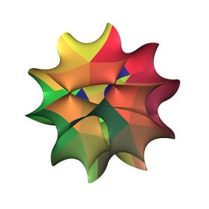
This is a visualization (actually a sort of “cross section”, since we can only display two dimensions and this object is actually six-dimensional) of the Calabi-Yau manifold described by the following polynomial equation:

This polynomial equation (known as the Fermat quintic) actually describes the Calabi-Yau manifold in projective space using homogeneous coordinates. This means that we are using the concepts of projective geometry (see Projective Geometry) to include “points at infinity“.
We note at this point that Kahler manifolds and Calabi-Yau manifolds are interesting in their own right, even outside of the context of string theory. For instance, we have briefly mentioned in Algebraic Cycles and Intersection Theory the Hodge conjecture, one of seven “Millenium Problems” for which the Clay Mathematics Institute is currently offering a million-dollar prize, and it concerns Kahler manifolds. Perhaps most importantly, it “unifies” several different branches of mathematics; as we have already seen, the study of Kahler manifolds and Calabi-Yau manifolds involves Riemannian geometry, symplectic geometry, complex geometry, and algebraic geometry. The more recent version of mirror symmetry called homological mirror symmetry further adds category theory and homological algebra to the mix.
Now what mirror symmetry more specifically states is that a version of string theory called Type IIA string theory, on a spacetime with extra dimensions compactified onto a certain Calabi-Yau manifold  , is the same as another version of string theory, called Type IIB string theory, on a spacetime with extra dimensions compactified onto another Calabi-Yau manifold
  , which is “mirror” to the Calabi-Yau manifold .
The statement of homological mirror symmetry (which is still conjectural, but mathematically proven in certain special cases) expresses the idea of the previous paragraph as follows (quoted verbatim from the paper Homological Algebra of Mirror Symmetry by Maxim Kontsevich):
Let  be a
be a  -dimensional symplectic manifold with
  and be a dual
  -dimensional complex algebraic manifold.
The derived category constructed from the Fukaya category  (or a suitably enlarged one) is equivalent to the derived category of coherent sheaves on a complex algebraic variety .
The statement makes use of the language of category theory and homological algebra (see Category Theory, More Category Theory: The Grothendieck Topos, Even More Category Theory: The Elementary Topos, Exact Sequences, More on Chain Complexes, and The Hom and Tensor Functors), but the idea that it basically expresses is that there exists a relation between the symplectic aspects of the Calabi-Yau manifold , as encoded in its Fukaya category, and the complex aspects of the Calabi-Yau manifold , as encoded in its category of coherent sheaves (see Sheaves and More on Sheaves). As we have said earlier, the subjects of algebraic geometry and complex geometry are closely related, and hence the language of sheaves show up in (and is an important part of) both subjects. The concept of derived categories, which generalize derived functors like the Ext and Tor functors, allow us to relate the two categories, which otherwise would be expressing different concepts. Inspired by string theory, therefore, we have now a deep and beautiful idea in geometry, relating its different aspects.
Is string theory the correct way towards a complete theory of quantum gravity, or the so-called “theory of everything”? As of the moment, we don’t know. Quantum gravity is a very difficult problem, and the scales involved are still far out of our reach – in order to probe smaller and smaller scales we need particle accelerators with higher and higher energies, and right now the technologies that we have are still very, very far from the scales which are relevant to quantum gravity. Still, it is hoped for that whatever we find in experiments in the near future, not only in the particle accelerators but also in the radio telescopes that look out into space, will at least guide us towards the correct path.
There are some who believe that, in the absence of definitive experimental evidence, mathematical beauty is our next best guide. And, without a doubt, string theory is related to, and has inspired, some very beautiful and very interesting mathematics, including that which we have discussed in this post. Still, physics, like all natural science, is empirical (based on evidence and observation), and hence it is ultimately physical evidence that will be the judge of correctness. It may yet turn out that string theory is wrong, and that it is a different theory which describes the fundamental physical laws of nature, or that it needs drastic modifications to its ideas. This will not invalidate the mathematics that we have described here, anymore than the discoveries of Copernicus invalidated the mathematics behind the astronomical model of Ptolemy – in fact this mathematics not only outlived the astronomy of Ptolemy, but served the theories of Copernicus, and his successors, just as well. Hence we cannot really say that the efforts of Ptolemy were wasted, since even though his scientific ideas were shown to be wrong, still his mathematical methods were found very useful by those who succeeded him. Thus, while our current technological limitations prohibit us from confirming or ruling out proposals for a theory of quantum gravity such as string theory, there is still much to be gained from such continued efforts on the part of theory, while experiment is still in the process of catching up.
Our search for truth continues. Meanwhile, we have beauty to cultivate.
References:
String Theory on Wikipedia
Mirror Symmetry on Wikipedia
Homological Mirror Symmetry on Wikipedia
Calabi-Yau Manifold on Wikipedia
Kahler Manifold on Wikipedia
Riemannian Geometry on Wikipedia
Symplectic Geometry on Wikipedia
Complex Geometry on Wikipedia
Fukaya Category on Wikipedia
Coherent Sheaf on Wikipedia
Derived Category on Wikipedia
Image by User Andrew J. Hanson of Wikipedia
Homological Algebra of Mirror Symmetry by Maxim Kontsevich
The Elegant Universe: Superstrings, Hidden Dimensions, and the Quest for the Ultimate Theory by Brian Greene
String Theory by Joseph Polchinski
String Theory and M-Theory: A Modern Introduction by Katrin Becker, Melanie Becker, and John Schwarz


![A=\mathbb{Z}_{p}[[u]]](https://s0.wp.com/latex.php?latex=A%3D%5Cmathbb%7BZ%7D_%7Bp%7D%5B%5Bu%5D%5D&bg=ffffff&fg=444444&s=0&c=20201002)


![\phi^{*}\mathcal{E}[1/I]\to\mathcal{E}[1/I]](https://s0.wp.com/latex.php?latex=%5Cphi%5E%7B%2A%7D%5Cmathcal%7BE%7D%5B1%2FI%5D%5Cto%5Cmathcal%7BE%7D%5B1%2FI%5D&bg=ffffff&fg=444444&s=0&c=20201002)


![\displaystyle R\Gamma_{\mathrm{et}}(\mathrm{Spec}(R)[1/p],\mathbb{Z}/p^{n})\cong (\Delta_{R/A}[1/d]/p^{n})^{\phi=1}](https://s0.wp.com/latex.php?latex=%5Cdisplaystyle+R%5CGamma_%7B%5Cmathrm%7Bet%7D%7D%28%5Cmathrm%7BSpec%7D%28R%29%5B1%2Fp%5D%2C%5Cmathbb%7BZ%7D%2Fp%5E%7Bn%7D%29%5Ccong+%28%5CDelta_%7BR%2FA%7D%5B1%2Fd%5D%2Fp%5E%7Bn%7D%29%5E%7B%5Cphi%3D1%7D&bg=ffffff&fg=444444&s=0&c=20201002)


![R=\mathbb{Z}[x_{1},\ldots,x_{n}]](https://s0.wp.com/latex.php?latex=R%3D%5Cmathbb%7BZ%7D%5Bx_%7B1%7D%2C%5Cldots%2Cx_%7Bn%7D%5D&bg=ffffff&fg=444444&s=0&c=20201002)


 . We also consider the real line, which we will think of as being “wrapped” over the circle, like a spring. We may think of this “spring” as casting a “shadow”, which is the circle. See also the following image by user Yonatan of Wikipedia:
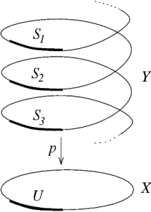
 with a continuous surjective map
  such that the “inverse image” of a small neighborhood in
  of
of  of
of 
 -dimensional real projective space
  (which is also known in the theory of Lie groups as
  ), whose universal covering space is the
  (which is also known as
  ). Similar to the above examples, we can think of
  .
. to
to  ; we may therefore also write it more suggestively as
![\displaystyle \int_{[a,b]}\frac{df}{dx}dx=f(b)-f(a)](https://s0.wp.com/latex.php?latex=%5Cdisplaystyle+%5Cint_%7B%5Ba%2Cb%5D%7D%5Cfrac%7Bdf%7D%7Bdx%7Ddx%3Df%28b%29-f%28a%29&bg=ffffff&fg=444444&s=0&c=20201002) .
.![[a,b]](https://s0.wp.com/latex.php?latex=%5Ba%2Cb%5D&bg=ffffff&fg=444444&s=0&c=20201002) . We denote the boundary of some “shape”
. We denote the boundary of some “shape”  by
by  . Therefore, in this case,
 ![\partial [a,b]=\{a\}\cup\{b\}](https://s0.wp.com/latex.php?latex=%5Cpartial+%5Ba%2Cb%5D%3D%5C%7Ba%5C%7D%5Ccup%5C%7Bb%5C%7D&bg=ffffff&fg=444444&s=0&c=20201002) .
.
 .
.
![\displaystyle \int_{[a,b]}df=f(b)-f(a)](https://s0.wp.com/latex.php?latex=%5Cdisplaystyle+%5Cint_%7B%5Ba%2Cb%5D%7Ddf%3Df%28b%29-f%28a%29&bg=ffffff&fg=444444&s=0&c=20201002) .
.
![\partial [a,b]=\{a\}^{-}\cup\{b\}^{+}](https://s0.wp.com/latex.php?latex=%5Cpartial+%5Ba%2Cb%5D%3D%5C%7Ba%5C%7D%5E%7B-%7D%5Ccup%5C%7Bb%5C%7D%5E%7B%2B%7D&bg=ffffff&fg=444444&s=0&c=20201002) , this now gives us the following expression for the fundamental theorem of calculus:
, this now gives us the following expression for the fundamental theorem of calculus:![\displaystyle \int_{[a,b]}df=\int_{\{a\}^{-}\cup\{b\}^{+}}f](https://s0.wp.com/latex.php?latex=%5Cdisplaystyle+%5Cint_%7B%5Ba%2Cb%5D%7Ddf%3D%5Cint_%7B%5C%7Ba%5C%7D%5E%7B-%7D%5Ccup%5C%7Bb%5C%7D%5E%7B%2B%7D%7Df&bg=ffffff&fg=444444&s=0&c=20201002)
![\displaystyle \int_{[a,b]}df=\int_{\partial [a,b]}f](https://s0.wp.com/latex.php?latex=%5Cdisplaystyle+%5Cint_%7B%5Ba%2Cb%5D%7Ddf%3D%5Cint_%7B%5Cpartial+%5Ba%2Cb%5D%7Df&bg=ffffff&fg=444444&s=0&c=20201002)

 ,
,  , and
, and  we will use
  ,
,  ,
,  , and so on. We will write exponents as
  , to hopefully avoid confusion.
 -forms by taking the wedge product. In ordinary multivariable calculus, the following expression

 ,
,  ,
,  , and
, and  . The wedge product expresses this same idea (in fact the wedge product
  is often also called the area form, mirroring the idea expressed by
  earlier), except that we want to include the concept of orientation that we discussed earlier. Therefore, in order to express this idea of orientation, we require the wedge product to satisfy the following property called antisymmetry:


 -forms, etc. using the wedge product. The collection of all these
  -forms.
 given by the following expression,
 , is given by
 .
. -form. We also note that the exterior derivative of an exterior derivative is always zero, i.e.
  for any differential form
 -form integrated over an
  form. Also, more rigorously the concept of integration on more complicated spaces involves the notion of “pullback”. We will leave these concepts to the references for now, contenting ourselves with the discussion of the wedge product and exterior derivative in this post. The application of differential forms to physics is discussed in the very readable book Gauge Fields, Knots and Geometry by John Baez and Javier P. Muniain.
 containing
  , called its vertices, such that the “difference vectors” defined by
  are linearly independent. We will use the notation
 ![[v_{0},...,v_{n}]](https://s0.wp.com/latex.php?latex=%5Bv_%7B0%7D%2C...%2Cv_%7Bn%7D%5D&bg=ffffff&fg=444444&s=0&c=20201002) to denote a simplex. We will keep track of the ordering of the vertices of the simplex, and we will always make use of the convention that the subscripts indexing the vertices are to be written in increasing order.
to denote a simplex. We will keep track of the ordering of the vertices of the simplex, and we will always make use of the convention that the subscripts indexing the vertices are to be written in increasing order. given by
 on the real line
  ), the standard
  ,
,  , and
, and  in
in  ,
,  ,
,  , and
, and  in
in 
![[v_{0},v_{1},v_{2}]](https://s0.wp.com/latex.php?latex=%5Bv_%7B0%7D%2Cv_%7B1%7D%2Cv_%7B2%7D%5D&bg=ffffff&fg=444444&s=0&c=20201002) . This is of course a triangle. To this
. This is of course a triangle. To this ![[v_{0},v_{1}]](https://s0.wp.com/latex.php?latex=%5Bv_%7B0%7D%2Cv_%7B1%7D%5D&bg=ffffff&fg=444444&s=0&c=20201002) ,
, ![[v_{1},v_{2}]](https://s0.wp.com/latex.php?latex=%5Bv_%7B1%7D%2Cv_%7B2%7D%5D&bg=ffffff&fg=444444&s=0&c=20201002) , and
, and ![[v_{0},v_{2}]](https://s0.wp.com/latex.php?latex=%5Bv_%7B0%7D%2Cv_%7B2%7D%5D&bg=ffffff&fg=444444&s=0&c=20201002) . They can be thought of as the “edges” of the
. They can be thought of as the “edges” of the ![\partial [v_{0},v_{1},v_{2}]](https://s0.wp.com/latex.php?latex=%5Cpartial+%5Bv_%7B0%7D%2Cv_%7B1%7D%2Cv_%7B2%7D%5D&bg=ffffff&fg=444444&s=0&c=20201002) .
. ) is given by
![\displaystyle \partial [v_{0},...,v_{n}]=\sum_{i}^{n}(-1)^{i}[v_{0},...,\hat{v_{i}},...,v_{n}]](https://s0.wp.com/latex.php?latex=%5Cdisplaystyle+%5Cpartial+%5Bv_%7B0%7D%2C...%2Cv_%7Bn%7D%5D%3D%5Csum_%7Bi%7D%5E%7Bn%7D%28-1%29%5E%7Bi%7D%5Bv_%7B0%7D%2C...%2C%5Chat%7Bv_%7Bi%7D%7D%2C...%2Cv_%7Bn%7D%5D&bg=ffffff&fg=444444&s=0&c=20201002)
 means that the vertex
  is to be omitted. Therefore, for the
 ![\partial[v_{0},v_{1},v_{2}]](https://s0.wp.com/latex.php?latex=%5Cpartial%5Bv_%7B0%7D%2Cv_%7B1%7D%2Cv_%7B2%7D%5D&bg=ffffff&fg=444444&s=0&c=20201002) is given by
is given by![\displaystyle \partial [v_{0},v_{1},v_{2}]=[v_{0},v_{1}]-[v_{0},v_{2}]+[v_{1},v_{2}]](https://s0.wp.com/latex.php?latex=%5Cdisplaystyle+%5Cpartial+%5Bv_%7B0%7D%2Cv_%7B1%7D%2Cv_%7B2%7D%5D%3D%5Bv_%7B0%7D%2Cv_%7B1%7D%5D-%5Bv_%7B0%7D%2Cv_%7B2%7D%5D%2B%5Bv_%7B1%7D%2Cv_%7B2%7D%5D&bg=ffffff&fg=444444&s=0&c=20201002) .
. endowed with an intuitive vector space structure. Given a point on the plane, we draw an “arrow” with its “tail” at the chosen origin of the plane and its “head” at the given point. We can then add and scale these arrows to obtain other arrows, hence, these arrows form a vector space. This “graphical” method of studying vectors (again in the sense of a quantity with magnitude and direction) is in fact one of the most common ways of introducing the concept of vectors in physics.
 , we obtain the notion of a fiber bundle. A vector space is therefore just a special case of a fiber bundle. In
  and boundary homomorphisms
  such that for all
  sends every element in
  .
.
 . Cycles in
  . Therefore, we can also state our “important principle” as follows:
 for all
  for all
  . The identity elements of
  ,
,  , and
, and  if necessary. We will also write
 is the inclusion function sending
  to
to  . In other words,
  sends
sends 
 is the “constant” function that sends any element in
  . In other words, the image of the function
  is the entirety of
 in
in 
 and “embeds” them into the abelian group of the integers
  if they are even, and to the element
  :
: .
.

 for all
  commute with the boundary homomorphisms
  and
and  , i.e.
 for all
  for all
  satisfy the conditions for them to form a chain map, i.e. they commute with the boundary homomorphisms in the sense shown above.
 -dimensional chains.
 are then given as the quotient of the group of cycles (kernels of the
  . Together with the appropriate coboundary morphisms, they form what is called a cochain complex.
 are defined, dually to the homology groups, as the quotient of the the group of cocycles (kernels of the
  of a space
 ![[S^{n},X]](https://s0.wp.com/latex.php?latex=%5BS%5E%7Bn%7D%2CX%5D&bg=ffffff&fg=444444&s=0&c=20201002) of homotopy classes of functions from the
of homotopy classes of functions from the  is called the fundamental group of
  , for a certain group
  .
.![\displaystyle \tilde{H}^{n}(X, G)\cong [X, K(G,n)]](https://s0.wp.com/latex.php?latex=%5Cdisplaystyle+%5Ctilde%7BH%7D%5E%7Bn%7D%28X%2C+G%29%5Ccong+%5BX%2C+K%28G%2Cn%29%5D&bg=ffffff&fg=444444&s=0&c=20201002)
 ” denotes an isomorphism of groups and the
  are the reduced cohomology groups, obtained by “dualizing” the augmented chain complex of reduced homology, which has

 consisting of a single point trivial. We have the following relation between the homology groups
  :
:
 be the topological space obtained by adjoining a disjoint basepoint to


 with respective basepoints
  and
and  , is the topological space, written
  , given by the quotient space
  under the identification
  . One can think of the space
  of two circles can be thought of as the “figure eight”.
 , given by the quotient space
  . What this means is that we take the cartesian product of
  , given by the quotient space
  under the identifications
  and
and  for any
  , where
 ![[0,1]](https://s0.wp.com/latex.php?latex=%5B0%2C1%5D&bg=ffffff&fg=444444&s=0&c=20201002) . When
. When  is the cylinder, and
  , given by the quotient space
  . This can be thought of as taking the suspension
  of the circle
  of an
of an  and an
  is homeomorphic to an
  -dimensional sphere
  .
. of a space
  and equipped with an appropriate topology called the compact-open topology.
![\displaystyle [\Sigma X, Y]\cong [X, \Omega Y]](https://s0.wp.com/latex.php?latex=%5Cdisplaystyle+%5B%5CSigma+X%2C+Y%5D%5Ccong+%5BX%2C+%5COmega+Y%5D&bg=ffffff&fg=444444&s=0&c=20201002)


 for
for 
 is a sequence of spaces
  with basepoints and basepoint-preserving maps
  . A spectrum
  is a prespectrum with adjoints
  which are homeomorphisms.