Rotations in Three Dimensions

In Rotating and Reflecting Vectors Using Matrices we learned how to express rotations in $2$ -dimensional space using certain special $2\times 2$ matrices which form a group (see Groups) we call the special orthogonal group in dimension $2$ , or $\text{SO}(2)$ (together with other matrices which express reflections, they form a bigger group that we call the orthogonal group in $2$ dimensions, or $\text{O}(2)$ ).

In this post, we will discuss rotations in $3$ -dimensional space. As we will soon see, notations in $3$ -dimensional space have certain interesting features not present in the $2$ -dimensional case, and despite being seemingly simple and mundane, play very important roles in some of the deepest aspects of fundamental physics.

We will first discuss rotations in $3$ -dimensional space as represented by the special orthogonal group in dimension $3$ , written as $\text{SO}(3)$ .

We recall some relevant terminology from Rotating and Reflecting Vectors Using Matrices. A matrix is called orthogonal if it preserves the magnitude of (real) vectors. The magnitude of the vector $v$ must be equal to the magnitude of the vector $Av$ , for a matrix $A$ , to be orthogonal. Alternatively, we may require, for the matrix $A$ to be orthogonal, that it satisfy the condition

$\displaystyle AA^{T}=A^{T}A=I$

where $A^{T}$ is the transpose of $A$ and $I$ is the identity matrix. The word “special” denotes that our matrices must have determinant equal to $1$ . Therefore, the group $\text{SO}(3)$ consists of the $3\times3$ orthogonal matrices whose determinant is equal to $1$ .

The idea of using the group $\text{SO}(3)$ to express rotations in $3$ -dimensional space may be made more concrete using several different formalisms.

One popular formalism is given by the so-called Euler angles. In this formalism, we break down any arbitrary rotation in $3$ -dimensional space into three separate rotations. The first, which we write here by $\varphi$ , is expressed as a counterclockwise rotation about the $z$ -axis. The second, $\theta$ , is a counterclockwise rotation about an $x$ -axis that rotates along with the object. Finally, the third, $\psi$ , is expressed as a counterclockwise rotation about a $z$ -axis that, once again, has rotated along with the object. For readers who may be confused, animations of these steps can be found among the references listed at the end of this post.

The matrix which expresses the rotation which is the product of these three rotations can then be written as

$\displaystyle g(\varphi,\theta,\psi) = \left(\begin{array}{ccc} \text{cos}(\varphi)\text{cos}(\psi)-\text{cos}(\theta)\text{sin}(\varphi)\text{sin}(\psi) & -\text{cos}(\varphi)\text{sin}(\psi)-\text{cos}(\theta)\text{sin}(\varphi)\text{cos}(\psi) & \text{sin}(\varphi)\text{sin}(\theta) \\ \text{sin}(\varphi)\text{cos}(\psi)+\text{cos}(\theta)\text{cos}(\varphi)\text{sin}(\psi) & -\text{sin}(\varphi)\text{sin}(\psi)+\text{cos}(\theta)\text{cos}(\varphi)\text{cos}(\psi) & -\text{cos}(\varphi)\text{sin}(\theta) \\ \text{sin}(\psi)\text{sin}(\theta) & \text{cos}(\psi)\text{sin}(\theta) & \text{cos}(\theta) \end{array}\right)$ .

The reader may check that, in the case that the rotation is strictly in the $x$ – $y$ plane, i.e. $\theta$ and $\psi$ are zero, we will obtain

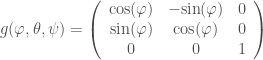$\displaystyle g(\varphi,\theta,\psi) = \left(\begin{array}{ccc} \text{cos}(\varphi) & -\text{sin}(\varphi) & 0 \\ \text{sin}(\varphi) & \text{cos}(\varphi) & 0 \\ 0 & 0 & 1 \end{array}\right)$ .

Note how the upper left part is an element of $\text{SO}(2)$ , expressing a counterclockwise rotation by an angle $\varphi$ , as we might expect.

Contrary to the case of $\text{SO}(2)$ , which is an abelian group, the group $\text{SO}(3)$ is not an abelian group. This means that for two elements $a$ and $b$ of $\text{SO}(3)$ , the product $ab$ may not always be equal to the product $ba$ . One can check this explicitly, or simply consider rotating an object along different axes; for example, rotating an object first counterclockwise by 90 degrees along the $z$ -axis, and then counterclockwise again by 90 degrees along the $x$ -axis, will not end with the same result as performing the same operations in the opposite order.

We now know how to express rotations in $3$ -dimensional space using $3\times 3$ orthogonal matrices. Now we discuss another way of expressing the same concept, but using “unitary”, instead of orthogonal, matrices. However, first we must revisit rotations in $2$ dimensions.

The group $\text{SO}(2)$ is not the only way we have of expressing rotations in $2$ -dimensions. For example, we can also make use of the unitary (we will explain the meaning of this word shortly) group in $1$ -dimension, also written $\text{U}(1)$ . It is the group formed by the complex numbers with magnitude equal to $1$ . The elements of this group can always be written in the form $e^{i\theta}$ , where $\theta$ is the angle of our rotation. As we have seen in Connection and Curvature in Riemannian Geometry, this group is related to quantum electrodynamics, as it expresses the gauge symmetry of the theory.

The groups $\text{SO}(2)$ and $\text{U}(1)$ are actually isomorphic. There is a one-to-one correspondence between the elements of $\text{SO}(2)$ and the elements of $\text{U}(1)$ which respects the group operation. In other words, there is a bijective function $f:\text{SO}(2)\rightarrow\text{U}(1)$ , which satisfies $ab=f(a)f(b)$ for $a$ , $b$ elements of $\text{SO}(2)$ . When two groups are isomorphic, we may consider them as being essentially the same group. For this reason, both $\text{SO}(2)$ and $U(1)$ are often referred to as the circle group.

We can now go back to rotations in $3$ dimensions and discuss the group $\text{SU}(2)$ , the special unitary group in dimension $2$ . The word “unitary” is in some way analogous to “orthogonal”, but applies to vectors with complex number entries.

Consider an arbitrary vector

$\displaystyle v=\left(\begin{array}{c}v_{1}\\v_{2}\\v_{3}\end{array}\right)$ .

An orthogonal matrix, as we have discussed above, preserves the quantity (which is the square of what we have referred to earlier as the “magnitude” for vectors with real number entries)

$\displaystyle v_{1}^{2}+v_{2}^{2}+v_{3}^{2}$

while a unitary matrix preserves

$\displaystyle v_{1}^{*}v_{1}+v_{2}^{*}v_{2}+v_{3}^{*}v_{3}$

where $v_{i}^{*}$ denotes the complex conjugate of the complex number $v_{i}$ . This is the square of the analogous notion of “magnitude” for vectors with complex number entries.

Just as orthogonal matrices must satisfy the condition

$\displaystyle AA^{T}=A^{T}A=I$ ,

unitary matrices are required to satisfy the condition

$\displaystyle AA^{\dagger}=A^{\dagger}A=I$

where $A^{\dagger}$ is the Hermitian conjugate of $A$ , a matrix whose entries are the complex conjugates of the entries of the transpose $A^{T}$ of $A$ .

An element of the group $\text{SU}(2)$ is therefore a $2\times 2$ unitary matrix whose determinant is equal to $1$ . Like the group $\text{SO}(3)$ , the group $\text{SU}(2)$ is also a group which is not abelian.

Unlike the analogous case in $2$ dimensions, the groups $\text{SO}(3)$ and $\text{SU}(2)$ are not isomorphic. There is no one-to-one correspondence between them. However, there is a homomorphism from $\text{SU}(2)$ to $\text{SO}(3)$ that is “two-to-one”, i.e. there are always two elements of $\text{SU}(2)$ that get mapped to the same element of $\text{SO}(3)$ under this homomorphism. Hence, $\text{SU}(2)$ is often referred to as a “double cover” of $\text{SO}(3)$ .

In physics, this concept underlies the weird behavior of quantum-mechanical objects called spinors (such as electrons), which require a rotation of 720, not 360, degrees to return to its original state!

The groups we have so far discussed are not “merely” groups. They also possesses another kind of mathematical structure. They describe certain shapes which happen to have no sharp corners or edges. Technically, such a shape is called a manifold, and it is the object of study of the branch of mathematics called differential geometry, which we have discussed certain basic aspects of in Geometry on Curved Spaces and Connection and Curvature in Riemannian Geometry.

For the circle group, the manifold that it describes is itself a circle. The elements of the circle group correspond to the points of the circle. The group $\text{SU}(2)$ is the surface of the $4$ – dimensional sphere, or what we call a $3$ -sphere (for those who might be confused by the terminology, recall that we are only considering the surface of the sphere, not the entire volume, and this surface is a $3$ -dimensional, not a $4$ -dimensional, object). The group $\text{SO}(3)$ is $3$ -dimensional real projective space, written $\mathbb{RP}^{3}$ . It is a manifold which can be described using the concepts of projective geometry (see Projective Geometry).

A group that is also a manifold is called a Lie group (pronounced like “lee”) in honor of the mathematician Marius Sophus Lie who pioneered much of their study. Lie groups are very interesting objects of study in mathematics because they bring together the techniques of group theory and differential geometry, which teaches us about Lie groups on one hand, and on the other hand also teaches us more about both group theory and differential geometry themselves.

References:

Orthogonal Group on Wikipedia

Rotation Group SO(3) on Wikipedia

Euler Angles on Wikipedia

Unitary Group on Wikipedia

Spinor on Wikipedia

Lie Group on Wikipedia

Real Projective Space on Wikipedia

Algebra by Michael Artin