The Arithmetic Site and the Scaling Site

January 25, 2018January 26, 2018 / Anton Hilado / Leave a comment

Introduction

In The Riemann Hypothesis for Curves over Finite Fields, we gave a rough outline of Andre Weil’s strategy to prove the analogue of the famous Riemann hypothesis for curves over finite fields. A rather natural question to ask would be, does this strategy give us any suggestions on how to take on the original Riemann hypothesis? We mentioned briefly in The Field with One Element that some mathematicians hope to find in the theory of the so-called “field with one element” something that will allow them to apply the ideas of Weil’s proof to the original Riemann hypothesis, by viewing the scheme $\text{Spec}(\mathbb{Z})$ as some kind of “curve” over the “field with one element”.

In this post we will consider something along similar lines, examining a kind of “space” to which we can apply an analogue of Weil’s strategy. This approach is due to the mathematicians Alain Connes and Caterina Consani, and makes use of the concepts of sites and toposes (see More Category Theory: The Grothendieck Topos and Even More Category Theory: The Elementary Topos). This is perhaps appropriate, since sites or toposes are often referred to as “generalized spaces”.

We recall from The Riemann Hypothesis for Curves over Finite Fields some aspects of Weil’s strategy. The object in consideration is a curve $C$ over a finite field $\mathbb{F}_{q}$ . In order to write down the zeta function for $C$ , we need to count the number of points over $\mathbb{F}_{q^{n}}$ , for every $n$ from $1$ to infinity. We can do this by counting the fixed points of powers of the Frobenius morphism. Explicitly this means taking intersection numbers of the diagonal and the divisor formed by integral linear combinations of powers of the Frobenius morphism on $\bar{C}\times_{\bar{\mathbb{F}}_{q}}\bar{C}$ , where $\bar{\mathbb{F}}_{q}$ is an algebraic closure of $\mathbb{F}_{q}$ (it is the direct limit of the directed system formed by all the $\mathbb{F}_{q^{n}}$ ) and $\bar{C}=C\otimes_{\mathbb{F}_{q}}\bar{\mathbb{F}}_{q}$ . The number of points of $\bar{\mathbb{F}}_{q}$ will be the same as the number of points of $C$ over $\mathbb{F}_{q^{n}}$ . Throughout this post we should keep these steps of Weil’s strategy in mind.

In order to transfer this strategy of Weil to the original Riemann hypothesis, Connes and Consani construct the arithmetic site, meant to be the analogue of $C$ , and the scaling site, meant to be the analogue of $\bar{C}$ . The intuition behind these constructions is that the points of the scaling site, which is the same as the points of the arithmetic site “over $\mathbb{R}_{+}^{\text{max}}$ “, is the same as the points of the “adele class space” $\mathbb{Q}^{\times}\backslash\mathbb{A}_{\mathbb{Q}}/\hat{\mathbb{Z}}^{\times}$ , which originally came up in earlier work of Connes where he constructed a quantum-mechanical system which gives Riemann’s prime-counting function (whose study provided the historical origin of the Riemann hypothesis), in the form of Weil’s “explicit formula”, as a quantum-mechanical trace formula! In essence this work restates the Riemann hypothesis in terms of mathematical language more commonly associated to physics, and is part of Connes’ pioneering work in noncommutative geometry, a new area of mathematics also closely related to physics, in particular quantum mechanics and quantum field theory. In the definition of the adele class space, $\mathbb{A}_{\mathbb{Q}}$ refers to the ring of adeles of $\mathbb{Q}$ (see Adeles and Ideles), while $\hat{\mathbb{Z}}$ refers to $\prod_{p}\mathbb{Z}_{p}$ , where $\mathbb{Z}_{p}$ are the $p$ -adic integers, which can be defined as the inverse limit of the inverse system formed by $\mathbb{Z}/p^{n}\mathbb{Z}$ .

The Arithmetic Site

We now proceed to discuss the arithmetic site. It is described as the pair $(\widehat{\mathbb{N}^{\times}},\mathbb{Z}_{\text{max}})$ , where $\widehat{\mathbb{N}^{\times}}$ a Grothendieck topos, which, as we may recall from More Category Theory: The Grothendieck Topos, is defined as a category equivalent to the category $\text{Sh}(\mathbf{C},J)$ of sheaves on a site $(\mathbf{C},J)$ . In the case of $\widehat{\mathbb{N}^{\times}}$ , $\mathbf{C}$ is the category with only one object, and whose morphisms correspond to the multiplicative monoid of nonzero natural numbers $\mathbb{N}^{\times}$ (we also use $\mathbb{N}^{\times}$ to denote this category, and $\mathbb{N}_{0}^{\times}$ to denote the category with one object and whose morphisms correspond to $\mathbb{N}^{\times}\cup\{0\}$ ), while $J$ is the indiscrete, or chaotic, Grothendieck topology, where all presheaves are also sheaves.

As part of the definition of the arithmetic site, we must also specify a structure sheaf. In this case is provided by $\mathbb{Z}_{\text{max}}$ , the semiring (a semiring is like a ring, but is only a monoid, and not a group, under the “addition” operation – a semiring is also sometimes called a “rig“, because it is a ring without the “n” – the negative elements, and the most common example is the natural numbers $\mathbb{N}$ with the usual addition and multiplication) whose elements are just the integers, together with $-\infty$ , but where the “addition” is provided by the “maximum” operation, and the “multiplication” is provided by the ordinary addition! With the arithmetic site thus defined, we denote it by $\mathcal{A}$ .

We digress for a while to discuss the semiring $\mathbb{Z}_{\text{max}}$ , as well as the closely related semirings $\mathbb{R}_{\text{max}}$ (defined similarly to $\mathbb{Z}_{\text{max}}$ , but with the real numbers instead of the integers), $\mathbb{R}_{+}^{\text{max}}$ (whose elements are the positive real numbers, with the addition given by the maximum operation, and the multiplication given by the ordinary multiplication), and the so-called Boolean semifield $\mathbb{B}$ (whose elements are $0$ and $1$ , with the addition again given by the maximum operation, and the multiplication again given by the ordinary multiplication). These semirings have origins in the area of mathematics known as tropical geometry, so named because one of its pioneers, Imre Simon, comes from Brazil, which is a tropical country. However, another source of inspiration is the work of the mathematical physicist Viktor Pavlovich Maslov in “semiclassical” quantum mechanics, where certain approximations could be made as the quantum mechanical systems being studied approached the classical limit. Maslov considered a “conjugated” addition

$\displaystyle \lim_{\epsilon\to 0}(x^{\frac{1}{\epsilon}}+y^{\frac{1}{\epsilon}})^{\epsilon}$

and this just happened to be the same as $\text{max}(x,y)$ .

Going back to the arithmetic site, we now discuss its points. Recall from Even More Category Theory: The Elementary Topos that a point of a topos (we discussed elementary toposes in that post, but this also applies to Grothendieck toposes) is defined by a geometric morphism from the topos $\mathfrak{P}$ of sheaves of sets on the singleton set (the set with a single element) to the topos. This refers to a pair of adjoint functors such that the left-adjoint is left-exact (preserves finite limits). Therefore, for the arithmetic site, a point $p$ is given by such a pair $p^{*}$ and $p_{*}$ such that $p^{*}:\widehat{\mathbb{N}^{\times}}\rightarrow\textbf{Sets}$ is left-exact. The point $p$ is also uniquely determined by the covariant functor $\mathscr{P}=p^{*}\circ\epsilon:\mathbb{N}^{\times}\rightarrow\textbf{Sets}$ where $\epsilon:\mathbb{N}^{\times}\rightarrow\widehat{\mathbb{N}^{\times}}$ is the Yoneda embedding.

There is an equivalence of categories between the category of points of the arithmetic site and the category of totally ordered groups which are isomorphic to the nontrivial subgroups of $(\mathbb{Q},\mathbb{Q}_{+})$ and injective morphisms of ordered groups. For such an ordered group $\textbf{H}$ we therefore have a point $\mathscr{P}_{\textbf{H}}$ . This gives us a correspondence with $\mathbb{Q}_{+}^{\times}\backslash\mathbb{A}_{\mathbb{Q}}^{f}/\hat{\mathbb{Z}}^{\times}$ (where $\mathbb{A}_{\mathbb{Q}}^{f}$ refers to the ring of finite adeles of $\mathbb{Q}$ , which is defined similarly to the ring of adeles of $\mathbb{Q}$ except that the infinite prime is not considered) because any such ordered group $\textbf{H}$ is of the form $\textbf{H}_{a}$ , the ordered group of all rational numbers $q$ such that $aq\in\hat{\mathbb{Z}}$ , for some unique $a\in \mathbb{A}_{\mathbb{Q}}^{f}/\hat{\mathbb{Z}}$ . We can also now describe the stalks of the structure sheaf $\mathbb{Z}_{\text{max}}$ at the point $\mathscr{P}_{\textbf{H}}$ ; it is isomorphic to the semiring $H_{\text{max}}$ , with elements given by the set $(\textbf{H}\cup\{-\infty\})$ , addition given by the maximum operation, and multiplication given by the ordinary addition.

The arithmetic site is analogous to the curve $C$ over the finite field $\mathbb{F}_{q}$ . As for the finite field $\mathbb{F}_{q}$ , its analogue is given by the Boolean semifield $\mathbb{B}$ mentioned earlier, which has “characteristic $1$ “, reminiscent of the field with one element (see The Field with One Element). Next we want to find the analogues of the algebraic closure $\bar{\mathbb{F}}_{q}$ , as well as the Frobenius morphism. The former is given by the semiring $\mathbb{R}_{+}^{\text{max}}$ , which contains $\mathbb{B}$ , while the latter is given by multiplicative group of the positive real numbers $\mathbb{R}_{+}^{\times}$ , as it is isomorphic to the group of automorphisms of $\mathbb{R}_{+}^{\text{max}}$ that keep $\mathbb{B}$ fixed.

But while we do know that the points of the arithmetic topos are given by geometric morphisms $p:\mathfrak{P}\rightarrow \widehat{\mathbb{N}^{\times}}$ and determined by contravariant functors $\mathscr{P}_{\textbf{H}}:\mathbb{N}^{\times}\rightarrow\textbf{Sets}$ , what do we mean by its “points over $\mathbb{R}_{+}^{\text{max}}$ “? A point of the arithmetic site “over $\mathbb{R}_{+}^{\text{max}}$ ” refers to the pair $(\mathscr{P}_{\textbf{H}},f_{\mathscr{P}}^{\#})$ , where $\mathscr{P}_{\textbf{H}}:\mathbb{N}^{\times}\rightarrow\textbf{Sets}$ as earlier, and $f_{\mathscr{P}_{\textbf{H}}}^{\#}:H_{\text{max}}\rightarrow\mathbb{R}_{+}^{\text{max}}$ (we recall that $H_{\text{max}}$ are the stalks of the structure sheaf $\mathbb{Z}_{\text{max}}$ ). The points of the arithmetic site over $\mathbb{R}_{+}^{\text{max}}$ include its points “over $\mathbb{B}$ “, which are what we discussed earlier, and mentioned to be in correspondence with $\mathbb{Q}_{+}^{\times}\backslash\mathbb{A}_{\mathbb{Q}}^{f}/\hat{\mathbb{Z}}^{\times}$ . But in addition, there are also other points of the arithmetic site over $\mathbb{R}_{+}^{\text{max}}$ which are in correspondence with $\mathbb{Q}_{+}^{\times}\backslash((\mathbb{A}_{\mathbb{Q}}^{f}/\hat{\mathbb{Z}}^{\times})\times\mathbb{R}_{+}^{\times})$ , just as $\mathbb{R}_{+}^{\text{max}}$ contains all of $\mathbb{B}$ but also other elements. Altogether, the points of the arithmetic site over $\mathbb{R}_{+}^{\text{max}}$ correspond to the disjoint union of $\mathbb{Q}_{+}^{\times}\backslash\mathbb{A}_{\mathbb{Q}}^{f}/\hat{\mathbb{Z}}^{\times}$ and $\mathbb{Q}_{+}^{\times}\backslash((\mathbb{A}_{\mathbb{Q}}^{f}/\hat{\mathbb{Z}}^{\times})\times\mathbb{R}_{+}^{\times})$ , which is $\mathbb{Q}^{\times}\backslash\mathbb{A}_{\mathbb{Q}}/\hat{\mathbb{Z}}^{\times}$ , the adele class space as mentioned earlier.

There is a geometric morphism $\Theta:\text{Spec}(\mathbb{Z})\rightarrow \widehat{\mathbb{N}_{0}^{\times}}$ (here $\widehat{\mathbb{N}_{0}^{\times}}$ is defined similarly to $\widehat{\mathbb{N}^{\times}}$ , but with $\mathbb{N}_{0}^{\times}$ in place of $\mathbb{N}^{\times}$ ) uniquely determined by

$\displaystyle \Theta^{*}:\mathbb{N}_{0}^{\times}\rightarrow \text{Sh}(\text{Spec}(\mathbb{Z}))$

which sends the single object of $\mathbb{N}_{0}^{\times}$ to the sheaf $\mathcal{S}$ on $\text{Spec}(\mathbb{Z})$ , which we now describe. Let $H_{p}$ denote the set of all rational numbers $q$ such that $a_{p}q$ is an element of $\hat{Z}$ , where $a_{p}$ is the adele with a $0$ for the $p$ -th component and $1$ for all other components. Then the sheaf $\mathcal{S}$ can be described in terms of its stalks $\mathcal{S}_{\mathscr{P}}$ , which are given by $H_{p}^{+}$ , the positive part of $H_{p}$ , and $\mathcal{S}_{0}$ , given by $\{0\}$ . The sections $\Gamma(U,\mathcal{S})$ are given by the maps $\xi:U\rightarrow \coprod_{p}H_{p}^{+}$ such that $\xi_{p}\neq 0$ for finitely many $p\in U$ .

The Scaling Site

Now that we have defined the arithmetic site, which is the analogue of $C$ , and the points of the arithmetic site over $\mathbb{R}_{+}^{\text{max}}$ , which is the analogue of the points of $C$ over the algebraic closure $\bar{\mathbb{F}}_{q}$ , we now proceed to define the scaling site, which is the analogue of $\bar{C}=C\otimes_{\mathbb{F}_{q}}\bar{\mathbb{F}}_{q}$ . The points of the scaling site are the same as the points of the arithmetic site over $\mathbb{R}_{+}^{\text{max}}$ , which is analogous to the points of $\bar{C}$ being the same as the points of $C$ over $\bar{\mathbb{F}}_{q}$ . But the importance of the scaling site lies in the fact that we can construct the analogue of a sheaf of rational functions on it, and a Riemann-Roch theorem, which, as we may recall from The Riemann Hypothesis for Curves over Finite Fields, it is also an important part of Weil’s proof.

The scaling site is once again given by a pair $([0,\infty)\rtimes\mathbb{N}^{\times},\mathcal{O})$ , where $[0,\infty)\rtimes\mathbb{N}^{\times}$ is a Grothendieck topos and $\mathcal{O}$ is a structure sheaf, but both are quite sophisticated constructions compared to the arithmetic site. To describe the Grothendieck topos $[0,\infty)\rtimes\mathbb{N}^{\times}$ we recall that it must be a category equivalent to the category $\text{Sh}(\mathbf{C},J)$ of sheaves on some site $(\mathbf{C},J)$ . Here $\mathbf{C}$ is the category whose objects are given by bounded open intervals $\Omega\subset [0,\infty)$ , including the empty interval $\null$ , and whose morphisms are given by

$\displaystyle \text{Hom}(\Omega,\Omega')=\{n\in\mathbb{N}^{\times}|n\Omega\subset\Omega'\}$

and in the special case that $\Omega$ is the empty interval $\null$ , we have

$\displaystyle \text{Hom}(\Omega,\Omega')=\{*\}$ .

The Grothendieck topology $J$ here is defined by the collection $K(\Omega)$ of all ordinary covers of $\Omega$ for any object $\Omega$ of the category $\mathbf{C}$ :

$\displaystyle \{\Omega_{i}\}_{i\in I}=\{\Omega_{i}\subset\Omega|\cup_{i}\Omega_{i}=\Omega\}$

Now we have to describe the structure sheaf $\mathcal{O}$ . We start by considering $\mathbb{Z}_{\text{max}}$ , the structure sheaf of the arithmetic site. By “extension of scalars” from $\mathbb{B}$ to $\mathbb{R}_{+}^{\text{max}}$ we obtain the reduced semiring $\mathbb{Z}_{\text{max}}\hat{\otimes}_{\mathbb{B}}\mathbb{R}_{+}^{\text{max}}$ . This is not yet the structure sheaf $\mathcal{O}$ , because the underlying category and Grothendieck topology for the scaling site is more complicated than the arithmetic site, and unlike the case for the arithmetic site, for the scaling site not every presheaf is a sheaf. So we must first “localize” $\mathbb{Z}_{\text{max}}\hat{\otimes}_{\mathbb{B}}\mathbb{R}_{+}^{\text{max}}$ , and this gives us the structure sheaf $\mathcal{O}$ .

Let us describe $\mathbb{Z}_{\text{max}}\hat{\otimes}_{\mathbb{B}}\mathbb{R}_{+}^{\text{max}}$ in more detail. Let $H$ be a rank $1$ subgroup of $\mathbb{R}$ . Then an element of $H_{\text{max}}\hat{\otimes}_{\mathbb{B}}\mathbb{R}_{+}^{\text{max}}$ is given by a Newton polygon $N\subset\mathbb{R}^{2}$ , which is the convex hull of the union of finitely many quadrants $(x_{j},y_{j}-Q)$ , where $Q=H\times\mathbb{R}_{+}$ and $(x_{j},y_{j})\in H\times R$ (a set is a convex set if it contains the line segment connecting any two of its points; the convex hull of a set is the smallest convex set that contains it). The Newton polygon $N$ is uniquely determined by the function

$\displaystyle \ell_{N}(\lambda)=\text{max}(\lambda x_{j}+y_{j})$

for $\lambda\in\mathbb{R}_{+}$ . This correspondence gives us an isomorphism between $H\hat{\otimes}_{\mathbb{B}}\mathbb{R}_{+}^{\text{max}}$ and $\mathcal{R}(H)$ , the semiring of convex, piecewise affine, continuous functions on $[0,\infty)$ with slopes in $H\subset\mathbb{R}$ and finitely many singularities, with the pointwise operations (function is a convex function if the points on and above its graph form a convex set).

Therefore, we can describe the sections $\Gamma(\Omega,\mathcal{O})$ of the structure sheaf $\mathcal{O}$ , for any bounded open interval $\Omega$ , as the set of all convex, piecewise affine, continuous functions from $\Omega$ to $\mathbb{R}_{\text{max}}$ with slopes in $\mathbb{Z}$ . We can also likewise describe the stalks of the structure sheaf $\mathcal{O}$ – for a point $\mathfrak{p}_{H}:[0,\infty)\rtimes\mathbb{N}^{\times}\rightarrow\textbf{Sets}$ associated to a rank 1 subgroup $H\subset\mathbb{R}$ , the stalk $\mathcal{O}_{\mathfrak{p}_{H}}$ is given by the semiring $\mathcal{R}_{H}$ of germs of $\mathbb{R}_{+}^{\text{max}}$ -valued, convex, piecewise affine, continuous functions with slope in $H$ . We also have points $\mathfrak{p}_{H}^{0}:[0,\infty)\rtimes\mathbb{N}^{\times}\rightarrow\textbf{Sets}$ with “support $\{0\}$ “, corresponding to the points of the arithmetic site over $\mathbb{B}$ . For such a point, the stalk $\mathcal{O}_{\mathfrak{p}_{H}^{0}}$ is given by the semiring $(H\times\mathbb{R})_{\text{max}}$ associated to the totally ordered group $H\times\mathbb{R}$ .

Now that we have decribed the Grothendieck topos $[0,\infty)\rtimes\mathbb{N}^{\times}$ and the structure sheaf $\mathcal{O}$ , we describe the scaling site as being given by the pair $([0,\infty)\rtimes\mathbb{N}^{\times},\mathcal{O})$ , and we denote it by $\hat{\mathcal{A}}$ .

Our next task, now that we have described the arithmetic site and the scaling site, is to find the analogue of the Riemann-Roch theorem. We start by noting that we have a sheaf of semifields $\mathcal{K}$ , defined by letting $\mathcal{K}(\Omega)$ be the semifield of fractions of $\mathcal{O}(\Omega)$ . For an element $f_{H}$ in the stalk $\mathcal{K}_{\mathfrak{p}_{H}}$ of $\mathcal{K}$ , we define its order as

$\displaystyle \text{Order}_{H}(f):=h_{+}-h_{-}$

where

$\displaystyle h_{\pm}:=\lim_{\epsilon\to 0_{\pm}}(f((1+\epsilon)H)-f(H))/\epsilon$

for $\epsilon\in\mathbb{R}_{+}$ .

We let $C_{p}$ be the set of all points $\mathfrak{p}_{H}:[0,\infty)\rtimes\mathbb{N}^{\times}\rightarrow\textbf{Sets}$ of the scaling site $\hat{\mathcal{A}}$ such that $H$ is isomorphic to $H_{p}$ . The $C_{p}$ are the analogues of the orbits of Frobenius. There is a topological isomorphism $\eta_{p}:\mathbb{R}_{+}^{\times}/p^{\mathbb{Z}}\rightarrow C_{p}$ . It is worth noting that the expression $\mathbb{R}_{+}^{\times}/p^{\mathbb{Z}}$ is reminiscent of the Tate uniformization of an elliptic curve (which generalizes the idea that an elliptic curve over the complex numbers forms a lattice in the complex plane to other complete fields besides the complex numbers – see The Moduli Space of Elliptic Curves).

We have a pullback sheaf $\eta_{p}^{*}(\mathcal{O}|_{C_{p}})$ , which we denote suggestively by $\mathcal{O}_{p}$ . It is the sheaf on $\mathbb{R}_{+}^{\times}/p^{\mathbb{Z}}$ whose sections are convex, piecewise affine, continuous functions with slopes in $H_{p}$ . We can consider the sheaf of quotients $\mathcal{K}_{p}$ of $\mathcal{O}_{p}$ and its global sections $f:\mathbb{R}_{+}^{\times}\rightarrow\mathbb{R}$ , which are piecewise affine, continuous functions with slopes in $H_{p}$ such that $f(p\lambda)=f(\lambda)$ for all $\lambda\in\mathbb{R}_{+}^{\times}$ . Defining

$\displaystyle \text{Order}_{\lambda}(f):=\text{Order}_{\lambda H_{p}}(f\circ\eta_{p}^{-1})$

we have the following property for any $f\in H^{0}(\mathbb{R}_{+}^{\times}/p^{\mathbb{Z}},\mathcal{K}_{p})$ (recall that the zeroth cohomology group $H^{0}(\mathbb{R}_{+}^{\times}/p^{\mathbb{Z}},\mathcal{K}_{p})$ is defined as the space of global sections of $\mathcal{K}_{p}$ ):

$\displaystyle \sum_{\lambda\in\mathbb{R}_{+}^{\times}/p^{\mathbb{Z}}}\text{Order}_{\lambda}(f)=0$

We now want to define the analogue of divisors on $C_{p}$ (see Divisors and the Picard Group). A divisor $D$ on $C_{p}$ is a section $C_{p}\rightarrow H$ , mapping $\mathfrak{p}_{H}\in C_{p}$ to $D(H)\in H$ , of the bundle of pairs $(H,h)$ , where $H\subset\mathbb{R}$ is isomorphic to $H_{p}$ , and $h\in H$ . We define the degree of a divisor $D$ as follows:

$\displaystyle \text{deg}(D)=\sum_{\mathfrak{p}\in C_{p}}D(H)$

Given a point $\mathfrak{p}_{H}\in C_{p}$ such that $H=\lambda H_{p}$ for some $\lambda\in\mathbb{R}_{+}^{*}$ , we have a map $\lambda^{-1}:H\rightarrow H_{p}$ . This gives us a canonical mapping

$\displaystyle \chi: H\rightarrow H_{p}/(p-1)H_{p}\simeq\mathbb{Z}/(p-1)\mathbb{Z}$

Given a divisor $D$ on $C_{p}$ , we define

$\displaystyle \chi(D):=\sum_{\frak{p}_{H}\in C_{p}}\chi(D(H))\in\mathbb{Z}/(p-1)\mathbb{Z}$

We have $\text{deg}(D)=0$ and $\chi(D)=0$ if and only if $D=(f)$ , for $f\in H^{0}(\mathbb{R}_{+}^{\times}/p^{\mathbb{Z}}\mathcal{K}_{p})$ i.e. $D$ is a principal divisor.

We define the group $J(C_{p})$ as the quotient $\text{Div}^{0}(C_{p})/\mathcal{P}$ of the group $\text{Div}^{0}(C_{p})$ of divisors of degree $0$ on $C_{p}$ by the group $\mathcal{P}$ of principal divisors on $C_{p}$ . The group $J(C_{p})$ is isomorphic to $\mathbb{Z}/(p-1)\mathbb{Z}$ , while the group $\text{Div}(C_{p})/\mathcal{P}$ of divisors on $C_{p}$ modulo the principal divisors is isomorphic to $\mathbb{R}\times(\mathbb{Z}/(p-1)\mathbb{Z})$ .

In order to state the analogue of Riemann-Roch theorem we need to define the following module over $\mathbb{R}_{+}^{\text{max}}$ :

$\displaystyle H^{0}(D):=\{f\in\mathcal{K}_{p}|D+(f)\geq 0\}$

Given $f\in H^{0}(C_{p},\mathcal{K}_{p})$ , we define

$\displaystyle \|f\|_{p}:=\text{max}\{h(\lambda)|_{p}/\lambda,\lambda\in C_{p}\}$

where $h(\lambda)$ is the slope of $f$ at $\lambda$ . Then we have the following increasing filtration on $H^{0}$ :

$\displaystyle H^{0}(D)^{\rho}:=\{f\in H^{0}(D)|\|f\|_{p}\leq\rho\}$

This allows us to define the following notion of dimension for $H^{0}(D)$ (here $\text{dim}_{\text{top}}$ refers to what is known as the topological dimension or Lebesgue covering dimension, a notion of dimension defined in terms of refinements of open covers):

$\displaystyle \text{Dim}_{\mathbb{R}}(H^{0}(D))=\lim_{n\to\infty}p^{-n}\text{dim}_{\text{top}}(H^{0}(D)^{p^{n}})$

The analogue of the Riemann-Roch theorem is now given by the following:

$\displaystyle \text{Dim}_{\mathbb{R}}(H^{0}(D))+\text{Dim}_{\mathbb{R}}(H^{0}(-D))=\text{deg}(D)$

S-Algebras

This concludes our discussion of the arithmetic site and the scaling site, but I would like to discuss one more related topic also being explored by Connes and Consani – the use of $\mathbb{S}$ -algebras, which is closely related to the $\Gamma$ -sets we have already introduced in The Field with One Element. Both of these concepts have their origins in homotopy theory.

We recall from the short discussion at the end of The Riemann Hypothesis for Curves over Finite Fields that the Weil conjectures, which are Weil’s generalization of the Riemann hypothesis for curves over finite fields to varieties of higher dimension, were proven by making use of cohomology (in particular etale cohomology) to find the fixed points of the powers of the Frobenius morphism (the formula that gives us the fixed points of a map using cohomology is called the Lefschetz fixed point formula). Now, concepts such as monoids, semirings, and many others (including the mathematician Nikolai Durov’s approach to the field with one element, which he also uses to develop a new version of Arakelov geometry) are all subsumed under the concept of $\mathbb{S}$ -algebras, and doing so allows us to make use of a cohomology theory called topological cyclic cohomology. Connes and Consani hope that topological cyclic cohomology will help prove the original Riemann hypothesis the way that etale cohomology helped prove the Weil conjectures. Let us discuss briefly the work of Connes and Consani on this topic.

We recall from The Field with One Element the definition of a $\Gamma$ -set (there also referred to as a $\Gamma$ -space). A $\Gamma$ -set is defined to be a covariant functor from the category $\Gamma^{\text{op}}$ , whose objects are pointed finite sets and whose morphisms are basepoint-preserving maps of finite sets, to the category $\textbf{Sets}_{*}$ of pointed sets. An $\mathbb{S}$ -algebra is defined to be a $\Gamma$ -set $\mathscr{A}:\Gamma^{\text{op}}\rightarrow \textbf{Sets}_{*}$ together with an associative multiplication $\mu:\mathscr{A}\wedge \mathscr{A}\rightarrow\mathscr{A}$ and a unit $1:\mathbb{S}\rightarrow\mathscr{A}$ , where $\mathbb{S}:\Gamma^{\text{op}}\rightarrow\textbf{Sets}_{*}$ is the inclusion functor (also known as the sphere spectrum). An $\mathbb{S}$ -algebra is a monoid in the symmetric monoidal category of $\Gamma$ -sets with the wedge product and the sphere spectrum.

Any monoid $M$ defines an $\mathbb{S}$ -algebra $\mathbb{S}M$ via the following definition:

$\displaystyle \mathbb{S}M(X):=M\wedge X$

for any pointed finite set $X$ . Here $M\wedge X$ is the smash product of $M$ and $X$ as pointed sets, with the basepoint for $M$ given by its zero element element. The maps are given by $\text{Id}_{M}\times f$ , for $f:X\rightarrow Y$ .

Similarly, any semiring $R$ defines an $\mathbb{S}$ -algebra $HR$ via the following definition:

$\displaystyle HR(X):=X^{R/*}$

for any pointed finite set $X$ . Here $X^{R/*}$ refers to the set of basepoint preserving maps from $R$ to $X$ . The maps $HR(f)$ are given by $HR(f)(\phi)(y):=\sum_{x\in f^{-1}(y)}\phi(x)$ for $f:X\rightarrow Y$ , $x\in X$ , and $y\in Y$ . The multiplication $HR(X)\wedge HR(Y)\rightarrow HR(X\wedge Y)$ is given by $\phi\psi(x,y)=\phi(x)\psi(y)$ for any $x\in X\setminus *$ and $y\in Y\setminus *$ . The unit $1_{X}:X\rightarrow HR(X)$ is given by $1_{X}(x)=\delta_{x}$ for all $x$ in $X$ , where $\delta_{x}(y)=1$ if $x=y$ , and $0$ otherwise.

Therefore we can see that the notion of $\mathbb{S}$ -algebra subsumes the notions of monoids and semirings, and other notions such as that of “hyperrings“, which we leave to the references for the moment. Instead, we will discuss how $\mathbb{S}$ -algebras are related to the approach of Durov to the field with one element and Arakelov geometry. As we mentioned in Arakelov Geometry, the main idea of the theory is to consider the “infinite prime” along with the other points of $\text{Spec}(\mathbb{Z})$ . We therefore define $\overline{\text{Spec}(\mathbb{Z})}$ as $\text{Spec}(\mathbb{Z})\cup \{\infty\}$ . Let $\mathcal{O}_{\text{Spec}(\mathbb{Z})}$ be the structure sheaf of $\text{Spec}(\mathbb{Z})$ . We want to extend this to a structure sheaf on $\overline{\text{Spec}(\mathbb{Z})}$ , and to accomplish this we will use the functor $H$ from semirings to $\mathbb{S}$ -algebras defined earlier. For any open set $U$ containing $\infty$ , we define

$\displaystyle \mathcal{O}_{\overline{\text{Spec}(\mathbb{Z})}}(U):=\|H\mathcal{O}_{\text{Spec}(\mathbb{Z})}(U\cup\text{Spec}(\mathbb{Z}))\|_{1}$ .

The notation $\|\|_{1}$ is defined for the $\mathbb{S}$ -algebra $HR$ associated to the semiring $R$ as follows:

$\displaystyle \|HR(X)\|_{1}:=\{\phi\in HR(X)|\sum_{X\*}\|\phi(x)\|\leq 1\}$

where $\|\|$ in this particular case comes from the usual absolute value on $\mathbb{Q}$ . This becomes available to us because the sheaf $\mathcal{O}_{\overline{\text{Spec}(\mathbb{Z})}}$ is a subsheaf of the constant sheaf $\mathbb{Q}$ .

Given an Arakelov divisor on $\overline{\text{Spec}(\mathbb{Z})}$ (in this context an Arakelov divisor is given by a pair $(D_{\text{finite}},D_{\infty})$ , where $D_{\text{finite}}$ is an ordinary divisor on $\text{Spec}(\mathbb{Z})$ and $D_{\infty}$ is a real number) we can define the following sheaf of $\mathcal{O}_{\overline{\text{Spec}(\mathbb{Z})}}$ -modules over $\overline{\text{Spec}(\mathbb{Z})}$ :

$\displaystyle \mathcal{O}_{\overline{\text{Spec}(\mathbb{Z})}}(D)(U):=\|H\mathcal{O}(D_{\text{finite}})(U\cup\text{Spec}(\mathbb{Z}))\|_{e^{a}}$

where $a$ is the real number “coefficient” of $D_{\infty}$ , and $\|\|_{\lambda}$ means, for an $R$ -module $E$ (here the $\mathbb{S}$ -algebra $HE$ is constructed the same as $HR$ , except there is no multiplication or unit) with seminorm $\|\|^{E}$ such that $\|a\xi\|^{E}\leq\|a\|\|\xi\|^{E}$ for $a\in R$ and $\xi\in E$ ,

$\displaystyle \|HE(X)\|_{\lambda}:=\{\phi\in HE(X)|^{E}\sum_{X\*}\|\phi(x)\|^{E}\leq \lambda\}$

With such sheaves of $\mathbb{S}$ -algebras on $\overline{\text{Spec}(\mathbb{Z})}$ now constructed, the tools of topological cyclic cohomology can be applied to it. The theory of topological cyclic cohomology is left to the references for now, but will hopefully be discussed in future posts on this blog.

Conclusion

The approach of Connes and Consani, whether making use of the arithmetic site and the scaling site to apply Weil’s strategy to the original Riemann hypothesis, or making use of $\mathbb{S}$ -algebras and topological cyclic cohomology in analogy with the proof of the Weil conjectures, is still currently facing several technical obstacles. In the former case, an intersection theory and a Riemann-Roch theorem on the square of the scaling site is yet to be constructed. In the latter, there is the problem of appropriate coefficients for the cohomology theory. There are already several proposed strategies for dealing with these obstacles. Such efforts, aside from aiming to prove the Riemann hypothesis, widens the scope of the mathematics that we have today, and, perhaps more importantly, uncovers more and more the mysterious geometry underlying the familiar everyday concept of numbers.

References:

On the Geometry of the Adele Class Space of Q by Caterina Consani

An Essay on the Riemann Hypothesis by Alain Connes

The Arithmetic Site by Alain Connes and Caterina Consani

Geometry of the Arithmetic Site by Alain Connes and Caterina Consani

The Scaling Site by Alain Connes and Caterina Consani

Geometry of the Scaling Site by Alain Connes and Caterina Consani

Absolute Algebra and Segal’s Gamma Sets by Alain Connes and Caterina Consani

New Approach to Arakelov Geometry by Nikolai Durov

The Riemann Hypothesis for Curves over Finite Fields

February 24, 2017July 6, 2017 / Anton Hilado / 8 Comments

The Riemann hypothesis is one of the most famous open problems in mathematics. Not only is there a million dollar prize currently being offered by the Clay Mathematical Institute for its solution, it also has a very long and interesting history spanning over a century and a half. It is part of many famous “lists” of open problems such as the famous 23 problems of David Hilbert, the 18 problems of Stephen Smale, and the 7 “millennium” problems of the aforementioned Clay Mathematical Institute.

The attention and reverence given to the Riemann hypothesis by the mathematical community is not without good reason. The problem originated in the paper “On the Number of Primes Less Than a Given Magnitude” by the mathematician Bernhard Riemann, where he applied the recently developed theory of complex analysis to number theory, in particular to come up with a function $\pi(x)$ that counts the number of prime numbers less than $x$ . The zeroes of the Riemann zeta function figure into the formula for this “prime counting function” $\pi(x)$ , and the Riemann hypothesis is a conjecture that concerns these zeroes. Aside from the knowledge about the prime numbers that a solution of the Riemann hypothesis will give us, it is hoped for that efforts toward this solution will lead to developments in mathematics that may be of interest to us for reasons much bigger, and perhaps outside of, the original motivations.

In the 1940’s, the mathematician Andre Weil solved a version of the Riemann hypothesis, which applies to the Riemann zeta function over finite fields. The ideas that Weil developed for solving this version of the Riemann hypothesis has led to many important developments in modern mathematics, whose applications are not limited to the original problem only. It is these ideas that we discuss in this post. But before we can give the statement of the Riemann hypothesis over finite fields (which is almost identical to that of the original Riemann hypothesis), we first review some concepts regarding zeta functions.

We have discussed zeta functions before in Zeta Functions and L-Functions. We recall that the Riemann zeta function is given by the formula

$\displaystyle \zeta(s)=\sum_{n=1}^{\infty}\frac{1}{n^{s}}$

or, in Euler product form,

$\displaystyle \zeta(s)=\prod_{p}\frac{1}{1-p^{-s}}$ .

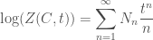
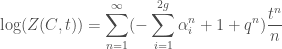
We now generalize the Riemann zeta function to any finitely generated ring $\mathcal{O}_{K}$ with field of fractions $K$ by writing it in the following form (this zeta function $\zeta(K,s)$ is also called the arithmetic zeta function):

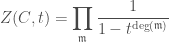
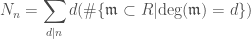
$\displaystyle \zeta(K,s)=\prod_{\mathfrak{m}}\frac{1}{1-(\# \mathcal{O}_{K}/\mathfrak{m})^{-s}}$

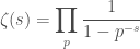
where $\mathfrak{m}$ runs over all the maximal ideals of the ring $\mathcal{O}_{K}$ , $\mathcal{O}_{K}/\mathfrak{m}$ is the residue field, and the expression $\#\mathcal{O}_{K}/\mathfrak{m}$ stands for the number of elements of this residue field. In the case that $\mathcal{O}_{K}=\mathbb{Z}$ , we get back our usual expression for the Riemann zeta function in its Euler product form, which we have written above, since the maximal ideals of $\mathbb{Z}$ are the principal ideals $(p)$ generated by the prime numbers, and the residue fields $\mathbb{Z}/(p)$ are the fields $\{0,1,...,p-1\}$ , therefore the number $\# \mathbb{Z}/(p)$ is equal to $p$ .

Next we discuss finite fields. All finite fields have a number of elements equal to some positive power of a prime number $p$ ; if this number is equal to $q=p^{n}$ , we write the finite field as $\mathbb{F}_{q}$ or $\mathbb{F}_{p^{n}}$ . In the case that $n=1$ , then $\mathbb{F}_{q}=\mathbb{F}_{p}$ is isomorphic to $\mathbb{Z}/p\mathbb{Z}$ .

Let $C$ be a nonsingular projective curve defined over the finite field $\mathbb{F}_{q}$ . “Nonsingular” roughly refers to the curve being “smooth”; or “differentiable”; “projective” roughly means that the curve is part, or a subset, of some projective space. We will not be dwelling too much on these technicalities in this post. “Defined over the finite field $\mathbb{F}_{q}$ ” means that the polynomial equation that defines the curve has coefficients which are elements of the finite field $\mathbb{F}_{q}$ . We know that in algebraic geometry (see Basics of Algebraic Geometry), the points of a curve (or more general varieties) correspond to maximal ideals of a “ring of functions” $\mathcal{O}_{K}$ on the curve $C$ . For a point $P$ on a curve over a finite field $\mathbb{F}_{q}$ , the residue field $\mathcal{O}_{K}/\mathfrak{m}$ , where $\mathfrak{m}$ is the maximal ideal corresponding to $P$ , is also a finite field of the form $\mathbb{F}_{q^{m}}$ . 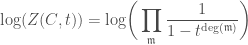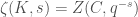The number $m$ is called the degree of $P$ and written $\text{deg}(P)$ , and we now define another zeta function (also called the local zeta function and written $Z(C,t))$ via the following formula:

$\displaystyle Z(C,t)=\prod_{P\in C}\frac{1}{1-t^{\text{deg}(P)}}$

or equivalently,

$\displaystyle Z(C,t)=\prod_{\mathfrak{m}}\frac{1}{1-t^{\text{deg}(\mathfrak{m})}}$ .

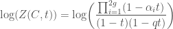
Note that this zeta function $Z(C,t)$ is related to the other zeta function $\zeta(K,s)$ by the following relation:

$\displaystyle \zeta(K,s)=Z(C,q^{-s})$ .

Next we take the “logarithm” of the zeta function $Z(C,t)$ . Using the familiar rules for taking the logarithms of products, we will obtain

$\displaystyle \text{log}(Z(C,t))=\text{log}\bigg(\prod_{\mathfrak{m}}\frac{1}{1-t^{\text{deg}(\mathfrak{m})}}\bigg)$

$\displaystyle \text{log}(Z(C,t))=\sum_{\mathfrak{m}}\text{log}\bigg(\frac{1}{1-t^{\text{deg}(\mathfrak{m})}}\bigg)$

$\displaystyle \text{log}(Z(C,t))=-\sum_{\mathfrak{m}}\text{log}\bigg(1-t^{\text{deg}(\mathfrak{m})}\bigg)$

Next we will need the following series expansion for logarithms:

$\displaystyle \text{log}(1-a)=-\sum_{k=0}^{\infty}\frac{a^{k}}{k}$ .

This allows us to write the logarithm of the zeta function as follows:

$\displaystyle \text{log}(Z(C,t))=\sum_{\mathfrak{m}}\sum_{k=1}^{\infty}\frac{(t^{\text{deg}(\mathfrak{m})})^{k}}{k}$

$\displaystyle \text{log}(Z(C,t))=\sum_{\mathfrak{m}}\sum_{k=1}^{\infty}\frac{(t^{\text{deg}(\mathfrak{m})})^{k}}{k\text{deg}(\mathfrak{m})}\text{deg}(\mathfrak{m})$

We can condense this expression by writing

$\displaystyle \text{log}(Z(C,t))=\sum_{n=1}^{\infty}N_{n}\frac{t^{n}}{n}$

where

$\displaystyle N_{n}=\sum_{d|n}d(\#\{\mathfrak{m}\subset R|\text{deg}(\mathfrak{m})=d\})$ .

The expression $d|n$ means “ $n$ is divisible by $d$ “, or “ $d$ divides $n$ “, which means that the sum is taken over all $d$ that divides $n$ .

The numbers $N_{n}$ can be thought of as the number of points on the curve $C$ whose coordinates are elements of the finite field $\mathbb{F}_{q^{n}}$ . In fact, we can actually define the zeta function $Z(C,t)$ starting with the numbers $N_{n}$ , i.e.

$\displaystyle Z(C,t)=\text{exp}\bigg(\sum_{n=1}^{\infty}N_{n}\frac{t^{n}}{n}\bigg)$

but we chose to start from the more familiar Riemann zeta function $\zeta(s)$ and generalize to get the form we want for curves over finite fields.

We recall that the zeroes of a function $f(z)$ are those $z_{i}$ such that $f(z_{i})=0$ .

We can now give the statement of the Riemann hypothesis for curves over finite fields:

The zeroes of the zeta function $\zeta(K,s)=Z(C,q^{-s})$ all have real part equal to $\frac{1}{2}$ .

We will not discuss the entirety of Weil’s proof in this post, although the reader may consult the references provided for such a discussion. Instead we will give a rough overview of Weil’s strategy, which rests on three important assumptions. We will show, roughly, how these assumptions lead to the proof of the Riemann hypothesis, and although we will not prove the assumptions themselves, we will also give a kind of preview of the ideas involved in their respective proofs. It is these ideas, which may now be considered to have developed into entire areas of research in themselves, which are perhaps the most enduring legacy of Weil’s proof.

Assumption 1 (Rationality): The zeta function $Z(C,t)$ can be written in the following form:

$\displaystyle Z(C,t)=\frac{\prod_{i=1}^{2g}(1-\alpha_{i}t)}{(1-t)(1-qt)}$

Given that this assumption holds, we can take the logarithm of the above expression,

$\displaystyle \text{log}(Z(C,t))=\text{log}\bigg(\frac{\prod_{i=1}^{2g}(1-\alpha_{i}t)}{(1-t)(1-qt)}\bigg)$

$\displaystyle \text{log}(Z(C,t))=\sum_{i=1}^{2g}\text{log}(1-\alpha_{i}t)-\text{log}(1-t)-\text{log}(1-qt)$

and we can then apply the series expansion for the logarithm that we have applied earlier to obtain the following expression,

$\displaystyle \text{log}(Z(C,t))=\sum_{n=1}^{\infty}(-\sum_{i=1}^{2g}\alpha_{i}^{n}+1+q^{n})\frac{t^{n}}{n}$

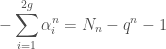
which we can now compare to the expression we obtained earlier for $\text{log}(Z(C,t))$ in terms of the number $N_{n}$ of points with coordinates in $\mathbb{F}_{q^{n}}$ :

$\displaystyle \sum_{n=1}^{\infty}(-\sum_{i=1}^{2g}\alpha_{i}^{n}+1+q^{n})\frac{t^{n}}{n}=\sum_{n=1}^{\infty}N_{n}\frac{t^{n}}{n}$ .

Comparing the coefficients of $\frac{t^{n}}{n}$ , we obtain, for each $n$ ,

$\displaystyle -\sum_{i=1}^{2g}\alpha_{i}^{n}+1+q^{n}=N_{n}$ .

With a little algebraic manipulation we have

$\displaystyle -\sum_{i=1}^{2g}\alpha_{i}^{n}=N_{n}-q^{n}-1$

and taking the absolute value of both sides gives us

$\displaystyle |\sum_{i=1}^{2g}\alpha_{i}^{n}|=|N_{n}-q^{n}-1|$

Assumption 2 (Hasse-Weil Inequality):

$\displaystyle |N_{n}-q^{n}-1|\leq 2gq^{\frac{n}{2}}$

This assumption, together with the earlier discussion, means that

$\displaystyle |\sum_{i=1}^{2g}\alpha_{i}^{n}|\leq 2gq^{\frac{n}{2}}$

We can then make use of the expansion

$\displaystyle \sum_{i=1}^{2g}\frac{1}{1-\alpha_{i}(q^{-\frac{1}{2}})}=\sum_{n=1}^{\infty}(\sum_{i=1}^{2g}\alpha_{i}^{n})(q^{-\frac{1}{2}})^{n}$

which in turn implies that

$|\alpha_{i}|\leq q^{\frac{1}{2}}$ for all $i$ from $1$ to $2g$ .

Assumption 3 (Functional Equation):

$\displaystyle Z\bigg(C,\frac{1}{qt}\bigg)=q^{1-g}t^{2-2g}Z(C,t)$

Given this assumption, and writing the zeta function $Z(C,t)$ explicitly, we have:

$\displaystyle \frac{\prod_{i=1}^{2g}(1-\alpha_{i}\frac{1}{qt})}{(1-\frac{1}{qt})(1-q\frac{1}{qt})}=q^{1-g}t^{2-2g}\frac{\prod_{i=1}^{2g}(1-\alpha_{i}t)}{(1-t)(1-qt)}$

With a little algebraic manipulation we can obtain the following equation:

$\displaystyle q^{g}t^{2g}\prod_{i=1}^{2g}(1-\alpha_{i}\frac{1}{qt})=\prod_{i=1}^{2g}(1-\alpha_{i}t)$

Let us write the product explicitly, and make the left side zero by letting $t=\frac{\alpha_{1}}{q}$ :

$\displaystyle q^{g}(\frac{\alpha_{1}}{q})^{2g}(0)(1-\alpha_{2}\frac{1}{q}\frac{q}{\alpha_{1}})...(1-\alpha_{2g}\frac{1}{q}\frac{q}{\alpha_{1}})=(1-\alpha_{1}\frac{\alpha_{1}}{q})(1-\alpha_{2}\frac{\alpha_{1}}{q})...(1-\alpha_{2g}\frac{\alpha_{1}}{q})$

Now since the left side is zero, the right side also must be zero. Therefore one of the factors in the product must be zero. This means that for some $i$ from $1$ to $2g$ , we have

$\displaystyle 1-\alpha_{i}\frac{\alpha_{1}}{q}=0$

In other words,

$\displaystyle \alpha_{i}\alpha_{1}=q$

This applies to any other $j$ from $1$ to $2g$ , not just $1$ , therefore more generally we must have

$\displaystyle \alpha_{i}\alpha_{j}=q$ for some $i$ and $j$ from $1$ to $2g$ .

If we combine this result with our earlier result that

$\displaystyle |\alpha_{i}|\leq q^{\frac{1}{2}}$ for all $i$ from $1$ to $2g$ ,

this means that

$\displaystyle |\alpha_{i}|=q^{\frac{1}{2}}$ for all $i$ from $1$ to $2g$ .

With this last result, we know that the zeroes of $Z(C,t)$ must have absolute value equal to $q^{-\frac{1}{2}}$ . Since $Z(C,q^{-s})=\zeta(K,s)$ , this implies that the real part of $s$ must be equal to $\frac{1}{2}$ , and this proves the Riemann hypothesis for curves over finite fields. More explicitly, let $t_{0}$ be a zero of the zeta function $Z(C,q^{-s})$ . We then have

$\displaystyle |t_{0}|=q^{-\frac{1}{2}}$

$\displaystyle |q^{-s}|=q^{-\frac{1}{2}}$

$\displaystyle |q^{-(\text{Re}(s)+\text{Im}(s))}|=q^{-\frac{1}{2}}$

$\displaystyle q^{-(\text{Re}(s))}=q^{-\frac{1}{2}}$

$\displaystyle \text{Re}(s)=\frac{1}{2}$

The proof of the rationality of the zeta function $Z(C,t)$ and the functional equation makes use of the theory of divisors (see Divisors and the Picard Group) and a very important theorem in algebraic geometry called the Riemann-Roch theorem. The Riemann-Roch theorem originates from complex analysis, which was the kind of the “specialty” of Bernhard Riemann (“On the Number of Primes Less Than a Given Magnitude” was his only paper on number theory, and it concerns the application of complex analysis to number theory). In its original formulation, the Riemann-Roch theorem gives the dimension of the vector space formed by the functions whose zeroes and poles (for a function which can be expressed as the ratio of two polynomials, the poles can be thought of as the zeroes of the denominator), and their “order of vanishing”, are specified. The Riemann-Roch theorem has since been generalized to aspects of algebraic geometry not necessarily directly concerned with complex analysis, and it is this generalization that allows us to make use of it for the case at hand.

In addition to the theory of divisors and the Riemann-Roch theorem, to prove the Hasse-Weil inequality, one must make use of the theory of fixed points, applied to what is known as the Frobenius morphism, which sends a point of $C$ with coordinates $a_{i}$ to the point with coordinates $a_{i}^{q}$ . The theory of fixed points is related to the part of algebraic geometry known as intersection theory. Roughly, given a function $f(x)$ , we can think of its fixed points as the values of $x$ for which $f(x)=x$ . One way to obtain these fixed points is to draw the graph of $y=x$ , and the graph of $y=f(x)$ , on the $x$ – $y$ plane; the fixed points of $f(x)$ are then given by the points where the two graphs intersect.

For the Frobenius morphism, the fixed points correspond to those points whose coordinates are elements of the finite field $\mathbb{F}_{q}$ . Similarly, the fixed points of the $n$ -th power of the Frobenius morphism (which we can think of as the Frobenius morphism applied $n$ times) correspond to those points whose coordinates are elements of the finite field $\mathbb{F}_{q^{n}}$ . Hence we can obtain the numbers $N_{n}$ that go into the expression of the zeta function $Z(C,t)$ using the Frobenius morphism. Combined with results from intersection theory such as the Castelnuovo-Severi inequality and the Hodge index theorem, this allows us to prove the Hasse-Weil inequality.

In algebraic geometry, curves are one-dimensional varieties, and just as there is a version of the Riemann hypothesis for curves over finite fields, there is also a version of the Riemann hypothesis for higher-dimensional varieties over finite fields, called the Weil conjectures, since they were proposed by Weil himself after he proved the case for curves. The Weil conjectures themselves follow the important assumptions involved in proving the Riemann hypothesis for curves over finite fields, such as the rationality of the zeta function and the functional equation. In addition, part of the Weil conjectures suggests a connection with the theory of cohomology (see Homology and Cohomology and Cohomology in Algebraic Geometry), which significant implications for the connections between algebraic geometry and methods originally developed for algebraic topology.

The Weil conjectures were proved by Bernard Dwork, Alexander Grothendieck, and Pierre Deligne. In his efforts to prove the Weil conjectures, Grothendieck developed the notion of topos (see More Category Theory: The Grothendieck Topos), as well as etale cohomology. As further part of his approach, Grothendieck also proposed conjectures, known as the standard conjectures on algebraic cycles, which remain open to this day. Grothendieck’s student, Pierre Deligne, was able to complete the proof of the Weil conjectures while bypassing the standard conjectures on algebraic cycles, by developing ingenious methods of his own. Still, the standard conjectures on algebraic cycles, as well as the related theory of motives, remain very much interesting on their own and continue to be a subject of modern mathematical research.

References:

Riemann Hypothesis on Wikipedia

Weil Conjectures on Wikipedia

Arithmetic Zeta Function on Wikipedia

Local Zeta Function on Wikipedia

The Weil Conjectures for Curves by Sam Raskin

Algebraic Geometry by Bas Edixhoven and Lenny Taelman

The Riemann Hypothesis over Finite Fields: From Weil to the Present Day by J.S. Milne

Algebraic Geometry by Robin Hartshorne