There are only four fundamental forces as far as we know, and every force that we know of can ultimately be considered as manifestations of these four. These four are electromagnetism, the weak nuclear force, the strong nuclear force, and gravity. Among them, the one we are most familiar with is electromagnetism, both in terms of our everyday experience (where it is somewhat on par with gravity) and in terms of our physical theories (where our understanding of electrodynamics is far ahead of our understanding of the other three forces, including, and especially, gravity).
Electromagnetism is dominant in everyday life because the weak and strong nuclear forces have a very short range, and because gravity is very weak. Now gravity doesn’t seem weak at all, especially if we have experienced falling on our face at some point in our lives. But that’s only because the “source” of this gravity, our planet, is very large. But imagine a small pocket-sized magnet lifting, say an iron nail, against the force exerted by the Earth’s gravity. This shows how much stronger the electromagnetic force is compared to gravity. Maybe we should be thankful that gravity is not on the same level of strength, or falling on our face would be so much more painful.
It is important to note also, that atoms, which make up everyday matter, are themselves made up of charged particles – electrons and protons (there are also neutrons, which are uncharged). Electromagnetism therefore plays an important part, not only in keeping the “parts” of an atom together, but also in “joining” different atoms together to form molecules, and other larger structures like crystals. It might be gravity that keeps our planet together, but for less massive objects like a house, or a car, or a human body, it is electromagnetism that keeps them from falling apart.
Aside from electromagnetism being the one fundamental force we are most familiar with, another reason to study it is that it is the “template” for our understanding of the rest of the fundamental forces, including gravity. In Einstein’s general theory of relativity, gravity is the curvature of spacetime; it appears that this gives it a nature different from the other fundamental forces. But even then, the expression for this curvature, in terms of the Riemann curvature tensor, is very similar in form to the equation for the electromagnetic fields in terms of the field strength tensor.
The electromagnetic fields, which we shall divide into the electric field and the magnetic field, are vector fields (see Vector Fields, Vector Bundles, and Fiber Bundles), which means that they have a value (both magnitude and direction) at every point in space. A charged particle in an electric or magnetic field (or both) will experience a force according to the Lorentz force law:
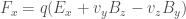
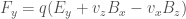

where 


The Lorentz force law is extremely important in electrodynamics and we will keep the following point in mind throughout this discussion:
The Lorentz force law tells us how charges move under the influence of electric and magnetic fields.
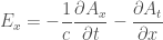
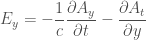
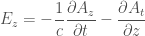
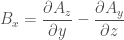
Instead of discussing electrodynamics in terms of these fields, however, we will instead focus on the electric and magnetic potentials, which together form what is called the four-potential and are related to the fields in terms of the following equations:


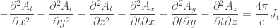
The values of the potentials, as functions of space and time, are related to the distribution of charges and currents by the very famous set of equations called Maxwell’s equations:


Some readers may be more familiar with Maxwell’s equations written in terms of the electric and magnetic fields; in that case, they have individual names: Gauss’ law, Gauss’ law for magnetism, Faraday’s law, and Ampere’s law (with Maxwell’s addition). When written down in terms of the fields, they can offer more physical intuition – for instance, Gauss’ law for magnetism tells us that the magnetic field has no “divergence”, and is always “solenoidal”. However, we leave this approach to the references for the moment, and focus on the potentials, which will be more useful for us when we relate our discussion to quantum mechanics later on. We will, however, always remind ourselves of the following important point:
Maxwell’s laws tells us the configuration and evolution of the electric and magnetic fields (possibly via the potentials) under the influence of sources (charge and current distributions).
There is one catch (an extremely interesting one) that comes about when dealing with potentials instead of fields. It is called gauge freedom, and is one of the foundations of modern particle physics. However, we will not discuss it in this post. Our equations will remain correct, so the reader need not worry; gauge freedom is not a constraint, but is instead a kind of “symmetry” that will have some very interesting consequences. This concept is left to the references for now, however it is hoped that it will at some time be discussed in this blog.
The way we have wrote down Maxwell’s equations is rather messy. However, we can introduce some notation to write them in a more elegant form. We use what is known as tensor notation; however we will not discuss the concept of tensors in full here. We will just note that because the formula for the spacetime interval contains a sign different from the others, we need two different types of indices for our vectors. The so-called contravariant vectors will be indexed by a superscript, while the so-called covariant vectors will be indexed by a subscript. “Raising” and “lowering” these indices will involve a change in sign for some quantities; we will indicate them explicitly here.
Let 


Let 


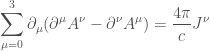
We now introduce the so-called Einstein summation convention. Note that the summation is performed over the index that is repeated; and that that one of these indices is a superscript and the other is a subscript. Albert Einstein noticed that almost all summations in his calculations happen in this way, so he adopted the convention that instead of explicitly writing out the summation sign, repeated indices (one superscript and one subscript) would instead indicate that a summation should be performed. Like most modern references, we adopt this notation, and only explicitly say so when there is an exception. This allows us to write Maxwell’s equations as
We can also use the Einstein summation convention to rewrite other important expressions in physics in more compact form. In particular, it allows us to rewrite the Dirac equation (see Some Basics of Relativistic Quantum Field Theory) as follows:
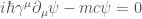
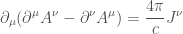
We now go to the quantum realm and discuss the equations of motion of quantum electrodynamics. Let 


What do these two equations mean?
The first equation looks like the Dirac equation, except that on the right hand side we have a term with both the “potential” (which we now call the Maxwell field, or the Maxwell field operator), the Dirac “wave function” for a particle such as an electron (which, as we have discussed in Some Basics of Relativistic Quantum Field Theory, is actually the Dirac field operator which operates on the “vacuum” state to describe a state with a single electron), as well as the charge. It describes the “motion” of the Dirac field under the influence of the Maxwell field. Hence, this is the quantum mechanical version of the Lorentz force law.
The second equation is none other than our shorthand version of Maxwell equations, and on the right hand side is an explicit expression for the current in terms of the Dirac field and some constants. The symbol 
In general relativity there is this quote, from the physicist John Archibald Wheeler: “Spacetime tells matter how to move; matter tells spacetime how to curve”. One can perhaps think of electrodynamics, whether classical or quantum, in a similar way. Fields tell charges and currents how to move, charges and currents tell fields how they are supposed to be “shaped”. And this is succinctly summarized by the Lorentz force law and Maxwell’s equations, again whether in its classical or quantum version.
As we have seen in Lagrangians and Hamiltonians, the equations of motion are not the only way we can express a physical theory. We can also use the language of Lagrangians and Hamiltonians. In particular, an important quantity in quantum mechanics that involves the Lagrangian and Hamiltonian is the probability amplitude. In order to calculate the probability amplitude, the physicist Richard Feynman developed a method involving the now famous Feynman diagrams, which can be though of as expanding the exponential function (see “The Most Important Function in Mathematics”) in the expression for the probability amplitude and expressing the different terms using diagrams. Just as we have associated the Dirac field to electrons, the Maxwell field is similarly associated to photons. Expressions involving the Dirac field and the Maxwell field can be thought of as electrons “emitting” or “absorbing” photons, or electrons and positrons (the antimatter counterpart of electrons) annihilating each other and creating a photon. The calculated probability amplitudes can then be used to obtain quantities that can be compared to results obtained from experiment, in order to verify the theory.
References:
Electromagnetic Four-Potential on Wikipedia
Maxwell’s Equations on Wikipedia
Quantum Electrodynamics on Wikipedia
Featured Image Produced by CERN
The Douglas Robb Memorial Lectures by Richard Feynman
QED: The Strange Theory of Light and Matter by Richard Feynman
Introduction to Electrodynamics by David J. Griffiths
Introduction to Elementary Particle Physics by David J. Griffiths
Quantum Field Theory by Fritz Mandl and Graham Shaw
Introduction to Quantum Field Theory by Michael Peskin and Daniel V. Schroeder
