In many posts on this blog, such as Basics of Arithmetic Geometry and Elliptic Curves, we have discussed how the geometry of shapes described by polynomial equations is closely related to number theory. This is especially true when it comes to the thousands-of-years-old subject of Diophantine equations, polynomial equations whose coefficients are whole numbers, and whose solutions of interest are also whole numbers (or, equivalently, rational numbers, since we can multiply or divide both sides of the polynomial equation by a whole number). We might therefore expect that the more modern and more sophisticated tools of algebraic geometry (which is a subject that started out as just the geometry of shapes described by polynomial equations) might be extremely useful in answering questions and problems in number theory.
One of the tools we can use for this purpose is the concept of an arithmetic scheme, which makes use of the ideas we discussed in Grothendieck’s Relative Point of View. An arithmetic variety is defined to be a a regular scheme that is projective and flat over the scheme  . An example of this is the scheme
 ![\text{Spec}(\mathbb{Z}[x])](https://s0.wp.com/latex.php?latex=%5Ctext%7BSpec%7D%28%5Cmathbb%7BZ%7D%5Bx%5D%29&bg=ffffff&fg=444444&s=0&c=20201002) , which is two-dimensional, and hence also referred to as an arithmetic surface.
, which is two-dimensional, and hence also referred to as an arithmetic surface.
We recall that the points of an affine scheme  , for some ring
  , are given by the prime ideals of . Therefore the scheme has one point for every prime ideal – one “closed point” for every prime number
  , and a “generic point” given by the prime ideal
  .
.
However, we also recall from Adeles and Ideles the concept of the “infinite primes” – which correspond to the archimedean valuations of a number field, just as the finite primes (primes in the classical sense) correspond to the nonarchimedean valuations. It is important to consider the infinite primes when dealing with questions and problems in number theory, and therefore we need to modify some aspects of algebraic geometry if we are to use it in helping us with number theory.
We now go back to arithmetic schemes, taking into consideration the infinite prime. Since we are dealing with the ordinary integers  , there is only one infinite prime, corresponding to the embedding of the rational numbers into the real numbers. More generally we can also consider an arithmetic variety over
  instead of , where
  is the ring of integers of a number field
  . In this case we may have several infinite primes, corresponding to the embediings of into the real and complex numbers. In this post, however, we will consider only and one infinite prime.
How do we describe an arithmetic scheme when the scheme has been “compactified” with the infinite prime? Let us look at the fibers of the arithmetic scheme. The fiber of an arithmetic scheme  at a finite prime is given by the scheme defined by the same homogeneous polynomials as , but with the coefficients taken modulo , so that they are elements of the finite field
  . The fiber over the generic point is given by taking the tensor product of the coordinate ring of with the rational numbers. But how should we describe the fiber over the infinite prime?
It was the idea of the mathematician Suren Arakelov that the fiber over the infinite prime should be given by a complex variety – in the case of an arithmetic surface, which Arakelov originally considered, the fiber should be given by a Riemann surface. The ultimate goal of all this machinery, at least when Arakelov was constructing it, was to prove the famous Mordell conjecture, which states that the number of rational solutions to a curve of genus greater than or equal to  was finite. These rational solutions correspond to sections of the arithmetic surface, and Arakelov’s strategy was to “bound” the number of these solutions by constructing a “height function” using intersection theory (see Algebraic Cycles and Intersection Theory) on the arithmetic surface. Arakelov unfortunately was not able to carry out his proof. He had only a very short career, being forced to retire after being diagnosed with schizophrenia. The Mordell conjecture was eventually proved by another mathematician, Gerd Faltings, who continues to develop Arakelov’s ideas.
Since we will be dealing with a complex variety, we must first discuss a little bit of differential geometry, in particular complex geometry (see An Intuitive Introduction to String Theory and (Homological) Mirror Symmetry). Let be a smooth projective complex equidimensional variety with complex dimension  . The space
  of differential forms (see Differential Forms) of degree
  on has the following decomposition:
We say that  is the vector space of complex-valued differential forms of type
  . We have differential operators

 .
.
 .
.
We let  be the dual to the vector space , and we write
  to denote
  . We refer to an element of
  as a current of type . We have an inclusion map

mapping a differential form  of type to a current
 ![[\omega]](https://s0.wp.com/latex.php?latex=%5B%5Comega%5D&bg=ffffff&fg=444444&s=0&c=20201002) of type , given by
of type , given by
=\int_{X}\omega\wedge\alpha](https://s0.wp.com/latex.php?latex=%5Cdisplaystyle+%5B%5Comega%5D%28%5Calpha%29%3D%5Cint_%7BX%7D%5Comega%5Cwedge%5Calpha&bg=ffffff&fg=444444&s=0&c=20201002)
for all  .
.
The differential operators  ,
,  , , and induce maps
  ,
,  , and
, and  on . We define the maps , , and on by


We also define
 .
.
For every irreducible analytic subvariety  of codimension , we define the current
  by
by
for all  , where
  is the nonsingular locus of
  .
.
A Green current  for a codimension analytic subvariety is defined to be an element of
  such that
![\displaystyle dd^{c}g+\delta_{Y}=[\omega]](https://s0.wp.com/latex.php?latex=%5Cdisplaystyle+dd%5E%7Bc%7Dg%2B%5Cdelta_%7BY%7D%3D%5B%5Comega%5D&bg=ffffff&fg=444444&s=0&c=20201002)
for some  .
.
Let  be the resolution of singularities of . This means that there exists a proper map
  such that
  is smooth,
  is a divisor with normal crossings (this means that each irreducible component of
  is nonsingular, and whenever they meet at a point their local equations are linearly independent) whenever
  contains the singular locus of , and
  is an isomorphism.
A smooth form  on
on  is said to be of logarithmic type along if there exists a projective map
  such that
  is a divisor with normal crossings,
  is smooth, and is the direct image by
  of a form
  on
on  satisfying the following equation

where  is a local equation of for every
  in ,
in ,  are and closed smooth forms, and
  is a smooth form.
For every irreducible subvariety there exists a smooth form  on of logarithmic type along such that
 ![[g_{Y}]](https://s0.wp.com/latex.php?latex=%5Bg_%7BY%7D%5D&bg=ffffff&fg=444444&s=0&c=20201002) is a Green current for :
is a Green current for :
![\displaystyle dd^{c}[g_{Y}]+\delta_{Y}=[\omega]](https://s0.wp.com/latex.php?latex=%5Cdisplaystyle+dd%5E%7Bc%7D%5Bg_%7BY%7D%5D%2B%5Cdelta_%7BY%7D%3D%5B%5Comega%5D&bg=ffffff&fg=444444&s=0&c=20201002)
where w is smooth on X. We say that is a Green current of logarithmic type.
We now proceed to discuss this intersection theory on the arithmetic scheme. We consider a vector bundle on the arithmetic scheme , a holomorphic vector bundle (a complex vector bundle  such that the projection map is holomorphic) on the fibers
  at the infinite prime, and a smooth hermitian metric (a sesquilinear form
  with the property that
  ) on which is invariant under the complex conjugation on . We refer to this collection of data as a hermitian vector bundle
  on .
on .
Given an arithmetic scheme and a hermitian vector bundle on , we can define associated “arithmetic”, or “Arakelov-theoretic” (i.e. taking into account the infinite prime) analogues of the algebraic cycles and Chow groups that we discussed in Algebraic Cycles and Intersection Theory.
An arithmetic cycle on is a pair  where
where  is an algebraic cycle on , i.e. a linear combination
  of closed irreducible subschemes
  of , of some fixed codimension , with integer coefficients
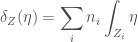
  , and is a Green current for , i.e. satisfies the equation
![\displaystyle dd^{c}g+\delta_{Z}=[\omega]](https://s0.wp.com/latex.php?latex=%5Cdisplaystyle+dd%5E%7Bc%7Dg%2B%5Cdelta_%7BZ%7D%3D%5B%5Comega%5D&bg=ffffff&fg=444444&s=0&c=20201002)
where
for differential forms and  of appropriate degree.
We define the arithmetic Chow group  as the group of arithmetic cycles
  modulo the subgroup
  generated by the pairs
  and
and  , where
  and
and  are currents of appropriate degree and
  is some rational function on some irreducible closed subscheme of codimension
  in .
in .
Next we want to have an intersection product on Chow groups, i.e. a bilinear pairing

We now define this intersection product. Let ![[Y,g_{Y}]\in\widehat{CH}^{p}(X)](https://s0.wp.com/latex.php?latex=%5BY%2Cg_%7BY%7D%5D%5Cin%5Cwidehat%7BCH%7D%5E%7Bp%7D%28X%29&bg=ffffff&fg=444444&s=0&c=20201002) and
and ![[Z,g_{Z}]\in\widehat{CH}^{q}](https://s0.wp.com/latex.php?latex=%5BZ%2Cg_%7BZ%7D%5D%5Cin%5Cwidehat%7BCH%7D%5E%7Bq%7D&bg=ffffff&fg=444444&s=0&c=20201002) . Assume that and are irreducible. Let
. Assume that and are irreducible. Let  , and
, and  . If
. If  and
and  intersect properly, i.e.
  , then we have
![\displaystyle [(Y,g_{Y})]\cdot [(Z,g_{Z})]:=[[Y]\cdot[Z],g_{Y}*g_{Z}]](https://s0.wp.com/latex.php?latex=%5Cdisplaystyle+%5B%28Y%2Cg_%7BY%7D%29%5D%5Ccdot+%5B%28Z%2Cg_%7BZ%7D%29%5D%3A%3D%5B%5BY%5D%5Ccdot%5BZ%5D%2Cg_%7BY%7D%2Ag_%7BZ%7D%5D&bg=ffffff&fg=444444&s=0&c=20201002)
where ![[Y]\cdot[Z]](https://s0.wp.com/latex.php?latex=%5BY%5D%5Ccdot%5BZ%5D&bg=ffffff&fg=444444&s=0&c=20201002) is just the usual intersection product of algebraic cycles, and
is just the usual intersection product of algebraic cycles, and  is the
  -product of Green currents, defined for a Green current of logarithmic type and a Green current
  , where and are closed irreducible subsets of with not contained in , as
![\displaystyle g_{Y}*g_{Z}:=[\tilde{g}_{Y}]*g_{Z}\text{ mod }(\text{im}(\partial)+\text{im}(\bar{\partial}))](https://s0.wp.com/latex.php?latex=%5Cdisplaystyle+g_%7BY%7D%2Ag_%7BZ%7D%3A%3D%5B%5Ctilde%7Bg%7D_%7BY%7D%5D%2Ag_%7BZ%7D%5Ctext%7B+mod+%7D%28%5Ctext%7Bim%7D%28%5Cpartial%29%2B%5Ctext%7Bim%7D%28%5Cbar%7B%5Cpartial%7D%29%29&bg=ffffff&fg=444444&s=0&c=20201002)
where
![\displaystyle [g_{Y}]*g_{Z}:=[g_{Y}]\wedge\delta_{Z}+[\omega_{Y}]\wedge g_{Z}](https://s0.wp.com/latex.php?latex=%5Cdisplaystyle+%5Bg_%7BY%7D%5D%2Ag_%7BZ%7D%3A%3D%5Bg_%7BY%7D%5D%5Cwedge%5Cdelta_%7BZ%7D%2B%5B%5Comega_%7BY%7D%5D%5Cwedge+g_%7BZ%7D&bg=ffffff&fg=444444&s=0&c=20201002)
and
![[g_{Y}]\wedge\delta_{Z}:=q_{*}[q^{*}g_{Y}]](https://s0.wp.com/latex.php?latex=%5Bg_%7BY%7D%5D%5Cwedge%5Cdelta_%7BZ%7D%3A%3Dq_%7B%2A%7D%5Bq%5E%7B%2A%7Dg_%7BY%7D%5D&bg=ffffff&fg=444444&s=0&c=20201002)
for  is the resolution of singularities of composed with the inclusion of into .
In the case that and  do not intersect properly, there is a rational function
  on
on  such that
  and intersect properly, and if
  is another rational function such that
  and intersect properly, the cycle

is in the subgroup . Here the notation  refers to the pair .
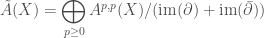
This concludes our little introduction to arithmetic intersection theory. We now give a short discussion what else can be done with such a theory. The mathematicians Henri Gillet and Christophe Soule used this arithmetic intersection theory to construct arithmetic analogues of Chern classes, Chern characters, Todd classes, and the Grothendieck-Riemann-Roch theorem (see Chern Classes and Generalized Riemann-Roch Theorems). These constructions are not so straightforward – for instance, one has to deal with the fact that unlike the classical case, the arithmetic Chern character is not additive on exact sequences. This failure to be additive on exact sequences is measured by the Bott-Chern character. The Bott-Chern character plays a part in defining the arithmetic analogue of the Grothendieck group  .
.
In order to define the arithmetic analogue of the Grothendieck-Riemann-Roch theorem, one must then define the direct image map  for a proper flat map
  of arithmetic varieties. This involves constructing a canonical line bundle
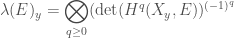
  on , whose fiber at
  is the determinant of cohomology of
  , i.e.
as well as a metric  , called the Quillen metric, on . With such a direct image map we can now give the statement of the arithmetic Grothendieck-Riemann-Roch theorem. It was originally stated by Gillet and Soule in terms of components of degree one in the arithmetic Chow group
  :
:

where  denotes the arithmetic Chern character,
  denotes the arithmetic Todd class,
  is the relative tangent bundle of ,
  is the map from
to  sending the element in
  to the class of
  in , and
 .
.
Later on Gillet and Soule formulated the arithmetic Grothendieck-Riemann-Roch theorem in higher degree as

for  .
.
Aside from the work of Gillet and Soule, there is also the work of the mathematician Amaury Thuillier making use of ideas from -adic geometry, constructing a nonarchimedean potential theory on curves that allows the finite primes and the infinite primes to be treated on a more equal footing, at least for arithmetic surfaces. The work of Thuillier is part of ongoing efforts to construct an adelic geometry, which is hoped to be the next stage in the evolution of Arakelov geometry.
References:
Arakelov Theory on Wikipedia
Arithmetic Intersection Theory by Henri Gillet and Christophe Soule
Theorie de l’Intersection et Theoreme de Riemann-Roch Arithmetiques by Jean-Benoit Bost
An Arithmetic Riemann-Roch Theorem in Higher Degrees by Henri Gillet and Christophe Soule
Theorie du Potentiel sur les Courbes en Geometrie Analytique Non Archimedienne et Applications a la Theorie d’Arakelov by Amaury Thuillier
Explicit Arakelov Geometry by Robin de Jong
Notes on Arakelov Theory by Alberto Camara
Lectures in Arakelov Theory by C. Soule, D. Abramovich, J.-F. Burnol, and J. Kramer
Introduction to Arakelov Theory by Serge Lang

 satisfying the condition that
 .
. , as is the case for the finite fields
  or
or  , therefore we will give more general forms for the equation of the elliptic curve later, along with the appropriate conditions. To help us with the latter, we will first look at the case of curves over the real numbers, where we can still make use of the equations above, and see what happens when the conditions on
  , in which case the condition is not satisfied. Then our curve (which is not an elliptic curve) is given by the equation

 and
and  . Once again the condition is not satisfied. Our curve is given by

 , the right hand side,
  , has a triple root at
  , while for
  , the right hand side,
  , factors into
  and therefore has a double root at
  .
.

 is a point with coordinates
  such that


 and
and  . The case
  of course corresponds to the “point at infinity”.
 . Then, since
  and
and  , we obtain the curve
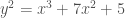
 . The right hand side actually factors into
 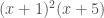 over
over  (which is equivalent to
  modulo
  ), and has discriminant equal to zero over
 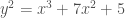 has bad reduction at
  ; in fact, we mentioned earlier that we cannot even write an elliptic curve in the form
  when the field of coefficients have characteristic equal to
  (where
  for some natural number
  . In our case, we are interested in the case
  , so that
  . When our elliptic curve has good reduction over
  , sometimes called the
  .
.
 if
if  if
if  if
if  if
if  , i.e. we have the following Taylor series expansion of the Hasse-Weil L-function at
 is the rank of the elliptic curve.
 are also the coefficients of the Fourier series expansion of some modular form
  (see
(see  .
. where
where  is the group of complex numbers of magnitude equal to
  with the law of composition given by the multiplication of complex numbers. When the complex points of the elliptic curve get mapped by the Weierstrass elliptic function to the points of the torus, the group structure provided by the “tangent and chord” or “tangent and secant” construction becomes the group structure of the torus. In other words, the Weierstrass elliptic function provides us with a group isomorphism.
 and
and  , a lattice
  in the complex plane is given by
 and
and  , gives a “square” lattice. This lattice is also the set of all Gaussian integers. The fundamental parallelogram is the parallelogram formed by the vertices
  . Here is an example of a lattice, courtesy of Alvaro Lozano-Robledo:

 , so that we have a new lattice equivalent under homothety to the old one, given by
 .
. , when written in polar form
  always has a positive angle
  between 0 and 180 degrees. If we cannot obtain this using our choice of
  , because of our convention in choosing
  . Several such complex numbers may refer to the same homothety class of lattices.
 refer to homothetic lattices if there exists the following relation between them:
 .
. matrix (see
  . It is the group of
  ,
,  ,
,  , and
, and  specify the same transformation, therefore what we actually want is the group called
  , also known as the modular group, and also written
  , obtained from the group
  , and then we identify two points if we can map one point into the other via the action of an element of the modular group, as we have discussed earlier. In technical language, we say that they belong to the same orbit. We can write our moduli space as
  (the notation means that the group
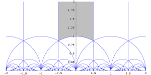
 ,
,  ,
,  , and
, and  , and
, and  ,
,  ,
,  . We will not discuss too much of these concepts for now. Instead we will give a preview of some concepts related to this moduli space. Topologically, this moduli space looks like a sphere with a missing point; in order to make the moduli space into a sphere (topologically), we take the union of the upper half plane
  . This projective line may be thought of as the set of all rational numbers
  (denoted
  by the same equivalence relation as earlier; this new space, topologically equivalent to the sphere, is called the modular curve
  .
.


 and
and  on the curve, we draw a line passing through both of them. In most cases, this line will pass through another point
  on the curve. This gives us the law of composition of the points of the elliptic curve, and we write
  . Here is an image courtesy of user SuperManu of Wikipedia:
 , the third point is
  , which is equal to
  , or
, or  . Again, since this necessitates taking a line that passes through the point
  , which is equal to
  .
. .
. , and hence we have written our law of composition “additively”.
 and
and  be the
  and
and  be the


 are given by the same formulas as above, appropriately modified to reflect the fact that now the points

 , we simply set
  , we set
  , reflecting its role as the identity element of the group.
 is isomorphic to the direct sum of
  over a field
  , the group of bijective linear transformations of the vector space
  for some prime number
  (see
(see  for integers