The Moduli Space of Elliptic Curves

A moduli space is a kind of “parameter space” that “classifies” mathematical objects. Every point of the moduli space stands for a mathematical object, in such a way that mathematical objects which are more similar to each other are closer and those that are more different from each other are farther apart. We may use the notion of equivalence relations (see Modular Arithmetic and Quotient Sets) to assign several objects which are in some sense “isomorphic” to each other to a single point.

We have discussed on this blog before one example of a moduli space – the projective line (see Projective Geometry). Every point on the projective line corresponds to a geometric object, a line through the origin. Two lines which have almost the same value of the slope will be closer on the projective line compared to two lines which are almost perpendicular.

Another example of a moduli space is that for circles on a plane – such a circle is specified by three real numbers, two coordinates for the center and one positive real number for the radius. Therefore the moduli space for circles on a plane will consist of a “half-volume” of some sort, like 3D space except that one coordinate is restricted to be strictly positive. But if we only care about the circles up to “congruence”, we can ignore the coordinates for the center – or we can also think of it as simply sending circles with the same radius to a single point, even if they are centered at different points. This moduli space is just the positive real line. Every point on this moduli space, which is a positive real number, corresponds to all the circles with radius equal to that positive real number.

We now want to construct the moduli space of elliptic curves. In order to do this we will need to first understand the meaning of the following statement:

Over the complex numbers, an elliptic curve is a torus.

We have already seen in Elliptic Curves what an elliptic curve looks like when graphed in the $x$ – $y$ plane, where $x$ and $y$ are real numbers. This gives us a look at the points of the elliptic curve whose coordinates are real numbers, or to put it in another way, these are the real numbers $x$ and $y$ which satisfy the equation of the elliptic curve.

When we look at the points of the elliptic curve with complex coordinates, or in other words the complex numbers which satisfy the equation of the elliptic curve, the situation is more complicated. First off, what we actually have is not what we usually think of as a curve, but rather a surface, in the same way that the complex numbers do not form a line like the real numbers do, but instead form a plane. However, even though it is not easy to visualize, there is a function called the Weierstrass elliptic function which provides a correspondence between the (complex) points of an elliptic curve and the points in the “fundamental parallelogram” of a lattice in the complex plane. We can think of “gluing” the opposite sides of this fundamental parallelogram to obtain a torus. This is what we mean when we say that an elliptic curve is a torus. This also means that there is a correspondence between elliptic curves and lattices in the complex plane.

We will discuss more about lattices later on in this post, but first, just in case the preceding discussion seems a little contrived, we elaborate a bit on the Weierstrass elliptic function. We must first discuss the concept of a holomorphic function. We have discussed in An Intuitive Introduction to Calculus the concept of the derivative of a function. Now not all functions have derivatives that exist at all points; in the case that the derivative of the function does exist at all points, we refer to the function as a differentiable function.

The concept of a holomorphic function in complex analysis (analysis is the term usually used in modern mathematics to refer to calculus and its related subjects) is akin to the concept of a differentiable function in real analysis. The derivative is defined as the limit of a certain ratio as the numerator and the denominator both approach zero; on the real line, there are limited ways in which these quantities can approach zero, but on the complex plane, they can approach zero from several different directions; for a function to be holomorphic, the expression for its derivative must remain the same regardless of the direction by which we approach zero.

In previous posts on topology on this blog we have been treating two different topological spaces as essentially the same whenever we can find a bijective and continuous function (also known as a homeomorphism) between them; similarly, we have been treating different algebraic structures such as groups, rings, modules, and vector spaces as essentially the same whenever we can find a bijective homomorphism (an isomorphism) between two such structures. Following these ideas and applying them to complex analysis, we may treat two spaces as essentially the same if we can find a bijective holomorphic function between them.

The Weierstrass elliptic function is not quite holomorphic, but is meromorphic – this means that it would have been holomorphic everywhere if not for the “lattice points” where there exist “poles”. But it is alright for us, because such a lattice point is to be mapped to the “point at infinity”. All in all, this allows us to think of the complex points of the elliptic curve as being essentially the same as a torus, following the ideas discussed in the preceding paragraph.

Moreover, the torus has a group structure of its own, considered as the direct product group $\text{U}(1)\times\text{U}(1)$ where $\text{U}(1)$ is the group of complex numbers of magnitude equal to $1$ with the law of composition given by the multiplication of complex numbers. When the complex points of the elliptic curve get mapped by the Weierstrass elliptic function to the points of the torus, the group structure provided by the “tangent and chord” or “tangent and secant” construction becomes the group structure of the torus. In other words, the Weierstrass elliptic function provides us with a group isomorphism.

All this discussion means that the study of elliptic curves becomes the study of lattices in the complex plane. Therefore, what we want to construct is the moduli space of lattices in the complex plane, up to a certain equivalence relation – two lattices are to be considered equivalent if one can be obtained by multiplying the other by a complex number (this equivalence relation is called homothety). Going back to elliptic curves, this corresponds to an isomorphism of elliptic curves in the sense of algebraic geometry.

Now given two complex numbers $\omega_{1}$ and $\omega_{2}$ , a lattice $\Lambda$ in the complex plane is given by

$\Lambda=\{m\omega_{1}+n\omega_{2}|m,n\in\mathbb{Z}\}$

For example, setting $\omega_{1}=1$ and $\omega_{2}=i$ , gives a “square” lattice. This lattice is also the set of all Gaussian integers. The fundamental parallelogram is the parallelogram formed by the vertices $0$ , $\omega_{1}$ , $\omega_{2}$ , and $\omega_{1}+\omega_{2}$ . Here is an example of a lattice, courtesy of Alvaro Lozano-Robledo:

The fundamental parallelogram is in blue. Here is another, courtesy of Sam Derbyshire:

Because we only care about lattices up to homothety, we can “rescale” the lattice by multiplying it with a complex number equal to $\frac{1}{\omega_{1}}$ , so that we have a new lattice equivalent under homothety to the old one, given by

$\Lambda=\{m+n\omega|m,n\in\mathbb{Z}\}$

where

$\displaystyle \tau=\frac{\omega_{2}}{\omega_{1}}$ .

We can always interchange $\omega_{1}$ and $\omega_{2}$ , but we will fix our convention so that the complex number $\tau=\frac{\omega_{2}}{\omega_{1}}$ , when written in polar form $\tau=re^{i\theta}$ always has a positive angle $\theta$ between 0 and 180 degrees. If we cannot obtain this using our choice of $\omega_{1}$ and $\omega_{2}$ , then we switch the two.

Now what this means is that a complex number $\omega$ , which we note is a complex number in the upper half plane $\mathbb{H}=\{z\in \mathbb{C}|\text{Im}(z)>0\}$ , because of our convention in choosing $\omega_{1}$ and $\omega_{2}$ , uniquely specifies a homothety class of lattices $\Lambda$ . However, a homothety class of lattices may not always uniquely specify such a complex number $\tau$ . Several such complex numbers may refer to the same homothety class of lattices.

What $\omega_{1}$ and $\omega_{2}$ specify is a choice of basis (see More on Vector Spaces and Modules) for the lattice $\Lambda$ ; we may choose several different bases to refer to the same lattice. Hence, the upper half plane is not yet the moduli space of all lattices in the complex plane (up to homothety); instead it is an example of what is called a Teichmuller space. To obtain the moduli space from the Teichmuller space, we need to figure out when two different bases specify lattices that are homothetic.

We will just write down the answer here; two complex numbers $\tau$ and $\tau'$ refer to homothetic lattices if there exists the following relation between them:

$\displaystyle \tau'=\frac{a\tau+b}{c\tau+d}$

for integers $a$ , $b$ , $c$ , and $d$ satisfying the identity

$\displaystyle ad-bc=1$ .

We can “encode” this information into a $2\times 2$ matrix (see Matrices) which is an element of the group (see Groups) called $\text{SL}(2,\mathbb{Z})$ . It is the group of $2\times 2$ matrices with integer entries and determinant equal to $1$ . Actually, the matrix with entries $a$ , $b$ , $c$ , and $d$ and the matrix with entries $-a$ , $-b$ , $-c$ , and $-d$ specify the same transformation, therefore what we actually want is the group called $\text{PSL}(2,\mathbb{Z})$ , also known as the modular group, and also written $\Gamma(1)$ , obtained from the group $\text{SL}(2,\mathbb{Z})$ by considering two matrices to be equivalent if one is the negative of the other.

We now have the moduli space that we want – we start with the upper half plane $\mathbb{H}$ , and then we identify two points if we can map one point into the other via the action of an element of the modular group, as we have discussed earlier. In technical language, we say that they belong to the same orbit. We can write our moduli space as $\Gamma(1)\backslash\mathbb{H}$ (the notation means that the group $\Gamma(1)$ acts on $\mathbb{H}$ “on the left”).

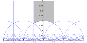
When dealing with quotient sets, which are sets of equivalence classes, we have seen in Modular Arithmetic and Quotient Sets that we can choose from an equivalence class one element to serve as the “representative” of this equivalence class. For our moduli space $\Gamma(1)\backslash\mathbb{H}$ , we can choose for the representative of an equivalence class a point from the “fundamental domain” for the modular group. Any point on the upper half plane can be obtained by acting on a point from the fundamental domain with an element of the modular group. The following diagram, courtesy of user Fropuff on Wikipedia, shows the fundamental domain in gray:

The other parts of the diagram show where the fundamental domain gets mapped to by certain special elements, in particular the “generators” of the modular group, which are the two elements where $a=0$ , $b=-1$ , $c=1$ , and $d=-1$ , and $a=1$ , $b=1$ , $c=1$ , and $d=0$ . We will not discuss too much of these concepts for now. Instead we will give a preview of some concepts related to this moduli space. Topologically, this moduli space looks like a sphere with a missing point; in order to make the moduli space into a sphere (topologically), we take the union of the upper half plane $\mathbb{H}$ with the projective line (see Projective Geometry) $\mathbb{P}^{1}(\mathbb{Q})$ . This projective line may be thought of as the set of all rational numbers $\mathbb{Q}$ together with a “point at infinity.” The modular group also acts on this projective line, so we can now take the quotient of $\mathbb{H}\cup\mathbb{P}^{1}(\mathbb{Q})$ (denoted $\mathbb{H}^{*}$ by the same equivalence relation as earlier; this new space, topologically equivalent to the sphere, is called the modular curve $X(1)$ .

The functions and “differential forms” on the modular curve $X(1)$ are of special interest. They can be obtained from functions on the upper half plane (with the “point at infinity”) satisfying certain conditions related to the modular group. If they are holomorphic everywhere, including the “point at infinity”, they are called modular forms. Modular forms are an interesting object of study in themselves, and their generalizations, automorphic forms, are a very active part of modern mathematical research.

Moduli Space on Wikipedia

Elliptic Curve on Wikipedia

Weierstrass’s Elliptic Functions on Wikipedia

Fundamental Pair of Periods on Wikipedia

Modular Group on Wikipedia

Fundamental Domain on Wikipedia

Modular Form on Wikipedia

Automorphic Form on Wikipedia

Image by Alvano Lozano Robledo on Wikipedia

Image by Sam Derbyshire on Wikipedia

Image by User Fropuff of Wikipedia

Advanced Topics in the Arithmetic of Elliptic Curves by Joseph H. Silverman